Hi all,I have successfully used the Object Detection API to train a model and am now trying to obtain a list of the class name and scores for the objects detected. Here is the code:
EDIT: Scores will not be required if the final output would only be a single class name. Thank you.
While this launches the cv2 display window successfully, I have been unable to find any workable solution to get class name or the score. Generally, I was unable to find no viable solutions at all, barring this one, but after trying the solution it has proven to unsuccessful too.
I hope that I can be pointed towards a tutorial for this, but any help/thoughts will be greatly appreciated.
Posted by Zizhao Zhang, Software Engineer, Google Cloud
In visual understanding, the Visual Transformer (ViT) and its variants have received significant attention recently due to their superior performance on many core visual applications, such as image classification, object detection, and video understanding. The core idea of ViT is to utilize the power of self-attention layers to learn global relationships between small patches of images. However, the number of connections between patches increases quadratically with image size. Such a design has been observed to be data inefficient — although the original ViT can perform better than convolutional networks with hundreds of millions of images for pre-training, such a data requirement is not always practical, and it still underperforms compared to convolutional networks when given less data. Many are exploring to find more suitable architectural re-designs that can learn visual representations effectively, such as by adding convolutional layers and building hierarchical structures with local self-attention.
The principle of hierarchical structure is one of the core ideas in vision models, where bottom layers learn more local object structures on the high-dimensional pixel space and top layers learn more abstracted and high-level knowledge at low-dimensional feature space. Existing ViT-based methods focus on designing a variety of modifications inside self-attention layers to achieve such a hierarchy, but while these offer promising performance improvements, they often require substantial architectural re-designs. Moreover, these approaches lack an interpretable design, so it is difficult to explain the inner-workings of trained models.
To address these challenges, in “Nested Hierarchical Transformer: Towards Accurate, Data-Efficient and Interpretable Visual Understanding”, we present a rethinking of existing hierarchical structure–driven designs, and provide a novel and orthogonal approach to significantly simplify them. The central idea of this work is to decouple feature learning and feature abstraction (pooling) components: nested transformer layers encode visual knowledge of image patches separately, and then the processed information is aggregated. This process is repeated in a hierarchical manner, resulting in a pyramid network structure. The resulting architecture achieves competitive results on ImageNet and outperforms results on data-efficient benchmarks. We have shown such a design can meaningfully improve data efficiency with faster convergence and provide valuable interpretability benefits. Moreover, we introduce GradCAT, a new technique for interpreting the decision process of a trained model at inference time.
Architecture Design The overall architecture is simple to implement by adding just a few lines of Python code to the source code of the original ViT. The original ViT architecture divides an input image into small patches, projects pixels of each patch to a vector with predefined dimension, and then feeds the sequences of all vectors to the overall ViT architecture containing multiple stacked identical transformer layers. While every layer in ViT processes information of the whole image, with this new method, stacked transformer layers are used to process only a region (i.e., block) of the image containing a few spatially adjacent image patches. This step is independent for each block and is also where feature learning occurs. Finally, a new computational layer called block aggregation then combines all of the spatially adjacent blocks. After each block aggregation, the features corresponding to four spatially adjacent blocks are fed to another module with a stack of transformer layers, which then process those four blocks jointly. This design naturally builds a pyramid hierarchical structure of the network, where bottom layers can focus on local features (such as textures) and upper layers focus on global features (such as object shape) at reduced dimensionality thanks to the block aggregation.
A visualization of the network processing an image: Given an input image, the network first partitions images into blocks, where each block contains 4 image patches. Image patches in every block are linearly projected as vectors and processed by a stack of identical transformer layers. Then the proposed block aggregation layer aggregates information from each block and reduces its spatial size by 4 times. The number of blocks is reduced to 1 at the top hierarchy and classification is conducted after the output of it.
Interpretability This architecture has a non-overlapping information processing mechanism, independent at every node. This design resembles a decision tree-like structure, which manifests unique interpretability capabilities because every tree node contains independent information of an image block that is being received by its parent nodes. We can trace the information flow through the nodes to understand the importance of each feature. In addition, our hierarchical structure retains the spatial structure of images throughout the network, leading to learned spatial feature maps that are effective for interpretation. Below we showcase two kinds of visual interpretability.
First, we present a method to interpret the trained model on test images, called gradient-based class-aware tree-traversal (GradCAT). GradCAT traces the feature importance of each block (a tree node) from top to bottom of the hierarchy structure. The main idea is to find the most valuable traversal from the root node at the top layer to a child node at the bottom layer that contributes the most to the classification outcomes. Since each node processes information from a certain region of the image, such traversal can be easily mapped to the image space for interpretation (as shown by the overlaid dots and lines in the image below).
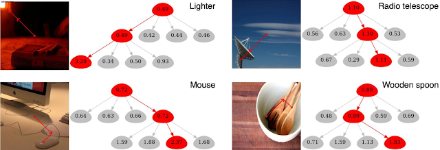
The following is an example of the model’s top-4 predictions and corresponding interpretability results on the left input image (containing 4 animals). As shown below, GradCAT highlights the decision path along the hierarchical structure as well as the corresponding visual cues in local image regions on the images.
Given the left input image (containing four objects), the figure visualizes the interpretability results of the top-4 prediction classes. The traversal locates the model decision path along the tree and simultaneously locates the corresponding image patch (shown by the dotted line on images) that has the highest impact to the predicted target class.
Moreover, the following figures visualize results on the ImageNet validation set and show how this approach enables some intuitive observations. For instance, the example of the lighter below (upper left panel) is particularly interesting because the ground truth class — lighter/matchstick — actually defines the bottom-right matchstick object, while the most salient visual features (with the highest node values) are actually from the upper-left red light, which conceptually shares visual cues with a lighter. This can also be seen from the overlaid red lines, which indicate the image patches with the highest impact on the prediction. Thus, although the visual cue is a mistake, the output prediction is correct. In addition, the four child nodes of the wooden spoon below have similar feature importance values (see numbers visualized in the nodes; higher indicates more importance), which is because the wooden texture of the table is similar to that of the spoon.
Visualization of the results obtained by the proposed GradCAT. Images are from the ImageNet validation dataset.
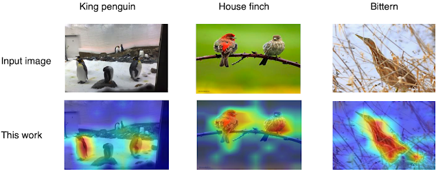
Second, different from the original ViT, our hierarchical architecture retains spatial relationships in learned representations. The top layers output low-resolution features maps of input images, enabling the model to easily perform attention-based interpretation by applying Class Attention Map (CAM) on the learned representations at the top hierarchical level. This enables high-quality weakly-supervised object localization with just image-level labels. See the following figure for examples.
Visualization of CAM-based attention results. Warmer colors indicate higher attention. Images are from the ImageNet validation dataset.
Convergence Advantages With this design, feature learning only happens at local regions independently, and feature abstraction happens inside the aggregation function. This design and simple implementation is general enough for other types of visual understanding tasks beyond classification. It also improves the model convergence speed greatly, significantly reducing the training time to reach the desired maximum accuracy.
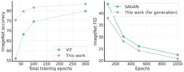
We validate this advantage in two ways. First, we compare the ViT structure on the ImageNet accuracy with a different number of total training epochs. The results are shown on the left side of the figure below, demonstrating much faster convergence than the original ViT, e.g., around 20% improvement in accuracy over ViT with 30 total training epochs.
Second, we modify the architecture to conduct unconditional image generation tasks, since training ViT-based models for image generation tasks is challenging due to convergence and speed issues. Creating such a generator is straightforward by transposing the proposed architecture: the input is an embedding vector, the output is a full image in RGB channels, and the block aggregation is replaced by a block de-aggregation component supported by Pixel Shuffling. Surprisingly, we find our generator is easy to train and demonstrates faster convergence speed, as well as better FID score (which measures how similar generated images are to real ones), than the capacity-comparable SAGAN.
Left: ImageNet accuracy given different number of total training epochs compared with standard ViT architecture. Right: ImageNet 64×64 image generation FID scores (lower is better) with single 1000-epoch training. On both tasks, our method shows better convergence speed.
Conclusion In this work we demonstrate the simple idea that decoupled feature learning and feature information extraction in this nested hierarchy design leads to better feature interpretability through a new gradient-based class-aware tree traversal method. Moreover, the architecture improves convergence on not only classification tasks but also image generation tasks. The proposed idea is focusing on aggregation function and thereby is orthogonal to advanced architecture design for self-attention. We hope this new research encourages future architecture designers to explore more interpretable and data-efficient ViT-based models for visual understanding, like the adoption of this work for high-resolution image generation. We have also released the source code for the image classification portion of this work.
Acknowledgements We gratefully acknowledge the contributions of other co-authors, including Han Zhang, Long Zhao, Ting Chen, Sercan Arik, Tomas Pfister. We also thank Xiaohua Zhai, Jeremy Kubica, Kihyuk Sohn, and Madeleine Udell for the valuable feedback of the work.
After meeting at an entrepreneur matchmaking event, Ulrik Hansen and Eric Landau teamed up to parlay their experience in financial trading systems into a platform for faster data labeling. In 2020, the pair of finance industry veterans founded Encord to adapt micromodels typical in finance to automated data annotation. Micromodels are neural networks that require Read article >
Read on how gradient descent and backpropagation algorithms relate to machine learning algorithms.
Artificial Neural Networks (ANN) are the fundamental building blocks of Artificial Intelligence (AI) technology. ANNs are the basis of machine-learning models; they simulate the process of learning identical to human brains. Simply put, ANNs give machines the capacity to accomplish human-like performance (and beyond) for specific tasks. This article aims to provide Data Scientists with the fundamental high-level knowledge of understanding the low-level operations involved in the functions and methods invoked when training an ANN.
As Data Scientists, we aim to solve business problems by exposing patterns in data. Often, this is done using machine learning algorithms to identify patterns and predictions expressed as a model . Selecting the correct model for a particular use case, and tuning parameters appropriately requires a thorough understanding of the problem and underlying algorithm(s). An understanding of the problem domain and the algorithms are taken under consideration to ensure that we are using the models appropriately, and interpreting results correctly.
This article introduces and explains gradient descent and backpropagation algorithms. These algorithms facilitate how ANNs learn from datasets, specifically where modifications to the network’s parameter values occur due to operations involving data points and neural network predictions.
Building an intuition
Before we get into the technical details of this post, let’s look at how humans learn.
The human brain’s learning process is complicated, and research has barely scratched the surface of how humans learn. However, the little that we do know is valuable and helpful for building models. Unlike machines, humans do not need a large quantity of data to comprehend how to tackle an issue or make logical predictions; instead, we learn from our experiences and mistakes.
Humans learn through a process of synaptic plasticity. Synaptic plasticity is a term used to describe how new neural connections are formed and strengthened after gaining new information. In the same way that the connections in the brain are strengthened and formed as we experience new events, we train artificial neural networks by computing the errors of neural network predictions and strengthening or weakening internal connections between neurons based on these errors.
Gradient Descent
Gradient Descent is a standard optimization algorithm. It is frequently the first optimization algorithm introduced to train machine learning. Let’s dissect the term “Gradient Descent” to get a better understanding of how it relates to machine learning algorithms.
A gradient is a measurement that quantifies the steepness of a line or curve. Mathematically, it details the direction of the ascent or descent of a line. Descent is the action of going downwards. Therefore, the gradient descent algorithm quantifies downward motion based on the two simple definitions of these phrases.
To train a machine learning algorithm, you strive to identify the weights and biases within the network that will help you solve the problem under consideration. For example, you may have a classification problem. When looking at an image, you want to determine if the image is of a cat or a dog. To build your model, you train your algorithm with training data with correctly labeled data samples of cats and dogs images.
While the example described above is classification, the problem could be localization or detection. Nonetheless, how well a neural network performs on a problem is modeled as a function, more specifically, a cost function; a cost or what is sometimes called a loss function measures how wrong a model is. The partial derivatives of the cost function influence the ultimate model’s weights and biases selected.
Gradient Descent is the algorithm that facilitates the search of parameters values that minimize the cost function towards a local minimum or optimal accuracy.
Cost functions, Gradient Descent and Backpropagation in Neural Networks
Neural networks are impressive. Equally impressive is the capacity for a computational program to distinguish between images and objects within images without being explicitly informed of what features to detect.
It is helpful to think of a neural network as a function that accepts inputs (data ), to produce an output prediction. The variables of this function are the parameters or weights of the neuron.
Therefore the key assignment to solving a task presented to a neural network will be to adjust the values of the weights and biases in a manner that approximates or best represents the dataset.
The image below depicts a simple neural network that receives input(X1, X2, X3, Xn), these inputs are fed forward to neurons within the layer containing weights(W1, W2, W3, Wn). The inputs and weights undergo a multiplication operation and the result is summed together by an adder(), and an activation function regulates the final output of the layer.
Figure 1: Image of a shallow neural network created by Author.
To assess the performance of neural networks, a mechanism for quantifying the difference or gap between the neural network prediction and the actual data sample value is required, yielding the calculation of a factor that influences the modification of weights and biases within a neural network.
The error gap between the predicted value of a neural network and the actual value of a data sample is facilitated by the cost function.
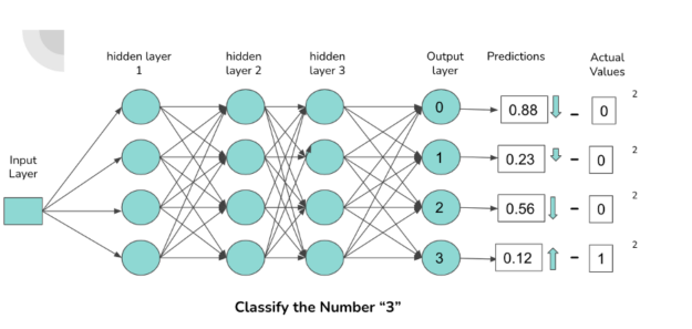
Figure 2: Neural Network internal connections and predictions depicted.
The image above illustrates a simple neural network architecture of densely connected neurons that classifies images containing the digits 0-3. Each neuron in the output layer corresponds to a digit. The higher the activations of the connection to a neuron, the higher the probability outputted by the neuron. The probability corresponds to the likelihood that the digit fed forward through the network is associated with the activated neuron.
When a ‘3’ is fed forward through the network, we expect the connections (represented by the arrows in the diagram) responsible for classifying a ‘3’ to have higher activation, which results in a higher probability for the output neuron associated with the digit ‘3’.
Several components are responsible for the activation of a neuron, namely biases, weights, and the previous layer activations. These specified components have to be iteratively modified for the neural network to perform optimally on a particular dataset.
By leveraging a cost function such as ‘mean squared error’, we obtain information in relation to the error of the network that is used to propagate updates backwards through the network’s weights and biases.
For completeness, below are examples of cost functions used within machine learning:
Mean Squared Error
Categorical Cross-Entropy
Binary Cross-Entropy
Logarithmic Loss
We have covered how to improve neural networks’ performance through a technique that measures the network’s predictions. The rest of the content in this article focuses on the relationship between gradient descent, backpropagation, and cost function.
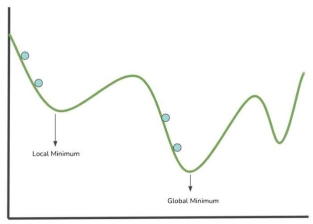
The image in figure 3 illustrates a cost function plotted on the x and y-axis that hold values within the function’s parameter space. Let’s take a look at how neural networks learn by visualizing the cost function as an uneven surface plotted on a graph within the parameter spaces of the possible weight/parameters values.
Figure 3: Gradient Descent visualized.
The blue points in the image above represent a step (evaluation of parameters values into the cost function) in the search for a local minimum. The lowest point of a modeled cost function corresponds to the position of weights values that results in the lowest value of the cost function. The smaller the cost function is, the better the neural network performs. Therefore, it is possible to modify the networks’ weights from the information gathered.
Gradient descent is the algorithm employed to guide the pairs of values chosen at each step towards a minimum.
Local Minimum: The minimum parameter values within a specified range or sector of the cost function.
Global Minimum: This is the smallest parameter value within the entire cost function domain.
The gradient descent algorithm guides the search for values that minimize the function at a local/global minimum by calculating the gradient of a differentiable function and moving in the opposite direction of the gradient.
Backpropagation is the mechanism by which components that influence the output of a neuron (bias, weights, activations) are iteratively adjusted to reduce the cost function. In the architecture of a neural network, the neuron’s input, including all the preceding connections to the neurons in the previous layer, determines its output.
The critical mathematical process involved in backpropagation is the calculation of derivatives. The backpropagation’s operations calculate the partial derivative of the cost function with respect to the weights, biases, and previous layer activations to identify which values affect the gradient of the cost function.
The minimization of the cost function by calculating the gradient leads to a local minimum. In each iteration or training step, the weights in the network are updated by the calculated gradient, alongside the learning rate, which controls the factor of modification made to weight values. This process is repeated for each step to be taken during the training phase of a neural network. Ideally, the goal is to be closer to a local minimum after each step.
The name “Backpropagation” comes from the process’s literal meaning, which is “backwards propagation of errors”. The partial derivative of the gradient quantifies the error. By propagating the errors backwards through the network, the partial derivative of the gradient of the last layer (closest layer to the output layer) is used to calculate the gradient of the second to the last layer.
The propagation of errors through the layers and the utilization of the partial derivative of the gradient from a previous layer in the current layer occurs until the first layer(closest layer to the input layer) in the network is reached.
Summary
This is just a primer on the topic of gradient descent. There is a whole world of mathematics and calculus associated with the topic of gradient descent.
Packages such as TensorFlow, SciKit-Learn, PyTorch often abstract the complexities of implementing training and optimization algorithms. Nevertheless, this does not relieve Data Scientists and ML practitioners of the requirement of understanding what occurs behind the scenes of these intelligent ‘black boxes.’
Want to explore more maths associated with backpropagation? Below are some resources to aid in your exploration:
I was interested as to how I could determine how much memory my saved neural network model requires. The reason I’m asking is that I’d like to test on an embedded device, and I’d like to see how much memory my current model takes first, and then I’d like to see how much memory my downsampled model requires next, and compare the performance reductions. Also, I have svm performing the same classification task, so I’m simply trying to figure out which is best for embedded devices.
Posted by Kevin Zakka, Student Researcher and Andy Zeng, Research Scientist, Robotics at Google
People learn to do things by watching others — from mimicking new dance moves, to watching YouTube cooking videos. We’d like robots to do the same, i.e., to learn new skillsbywatching people do things during training. Today, however, the predominant paradigm for teaching robots is to remote control them using specialized hardware for teleoperation and then train them to imitate pre-recorded demonstrations. This limits both who can provide the demonstrations (programmers & roboticists) and where they can be provided (lab settings). If robots could instead self-learn new tasks by watching humans, this capability could allow them to be deployed in more unstructured settings like the home, and make it dramatically easier for anyone to teach or communicate with them, expert or otherwise. Perhaps one day, they might even be able to use Youtube videos to grow their collection of skills over time.
Our motivation is to have robots watch people do tasks, naturally with their hands, and then use that data as demonstrations for learning. Video by Teh Aik Hui and Nathaniel Lim. License: CC-BY
However, an obvious but often overlooked problem is that a robot is physically different from a human, which means it often completes tasks differently than we do. For example, in the pen manipulation task below, the hand can grab all the pens together and quickly transfer them between containers, whereas the two-fingered gripper must transport one at a time. Priorresearchassumes that humans and robots can do the same task similarly, which makes manually specifying one-to-one correspondences between human and robot actions easy. But with stark differences in physique, defining such correspondences for seemingly easy tasks can be surprisingly difficult and sometimes impossible.
Physically different end-effectors (i.e., “grippers”) (i.e., the part that interacts with the environment) induce different control strategies when solving the same task. Left: The hand grabs all pens and quickly transfers them between containers. Right: The two-fingered gripper transports one pen at a time.
In “XIRL: Cross-Embodiment Inverse RL”, presented as an oral paper at CoRL 2021, we explore these challenges further and introduce a self-supervised method for Cross-embodiment Inverse Reinforcement Learning (XIRL). Rather than focusing on how individual human actions should correspond to robot actions, XIRL learns the high-level task objective from videos, and summarizes that knowledge in the form of a reward function that is invariant to embodiment differences, such as shape, actions and end-effector dynamics. The learned rewards can then be used together with reinforcement learning to teach the task to agents with new physical embodiments through trial and error. Our approach is general and scales autonomously with data — the more embodiment diversity presented in the videos, the more invariant and robust the reward functions become. Experiments show that our learned reward functions lead to significantly more sample efficient (roughly 2 to 4 times) reinforcement learning on new embodiments compared to alternative methods. To extend and build on our work, we are releasing an accompanying open-source implementation of our method along with X-MAGICAL, our new simulated benchmark for cross-embodiment imitation.
Cross-Embodiment Inverse Reinforcement Learning (XIRL) The underlying observation in this work is that in spite of the many differences induced by different embodiments, there still exist visual cues that reflect progression towards a common task objective. For example, in the pen manipulation task above, the presence of pens in the cup but not the mug, or the absence of pens on the table, are key frames that are common to different embodiments and indirectly provide cues for how close to being complete a task is. The key idea behind XIRL is to automatically discover these key moments in videos of different length and cluster them meaningfully to encode task progression. This motivation shares many similarities with unsupervised video alignment research, from which we can leverage a method called Temporal Cycle Consistency (TCC), which aligns videos accurately while learning useful visual representations for fine-grained video understanding without requiring any ground-truth correspondences.
We leverage TCC to train an encoder to temporally align video demonstrations of different experts performing the same task. The TCC loss tries to maximize the number of cycle-consistent frames (or mutual nearest-neighbors) between pairs of sequences using a differentiable formulation of soft nearest-neighbors. Once the encoder is trained, we define our reward function as simply the negative Euclidean distance between the current observation and the goal observation in the learned embedding space. We can subsequently insert the reward into a standard MDP and use an RL algorithm to learn the demonstrated behavior. Surprisingly, we find that this simple reward formulation is effective for cross-embodiment imitation.
XIRL self-supervises reward functions from expert demonstrations using temporal cycle consistency (TCC), then uses them for downstream reinforcement learning to learn new skills from third-person demonstrations.
X-MAGICAL Benchmark To evaluate the performance of XIRL and baseline alternatives (e.g., TCN, LIFS, Goal Classifier) in a consistent environment, we created X-MAGICAL, which is a simulated benchmark for cross-embodiment imitation. X-MAGICAL features a diverse set of agent embodiments, with differences in their shapes and end-effectors, designed to solve tasks in different ways. This leads to differences in execution speeds and state-action trajectories, which poses challenges for current imitation learning techniques, e.g., ones that use time as a heuristic for weak correspondences between two trajectories. The ability to generalize across embodiments is precisely what X-MAGICAL evaluates.
The SweepToTop task we considered for our experiments is a simplified 2D equivalent of a common household robotic sweeping task, where an agent has to push three objects into a goal zone in the environment. We chose this task specifically because its long-horizon nature highlights how different agent embodiments can generate entirely different trajectories (shown below). X-MAGICAL features a Gym API and is designed to be easily extendable to new tasks and embodiments. You can try it out today with pip install x-magical.
Different agent shapes in the SweepToTop task in the X-MAGICAL benchmark need to use different strategies to reposition objects into the target area (pink), i.e., to “clear the debris”. For example, the long-stick can clear them all in one fell swoop, whereas the short-stick needs to do multiple consecutive back-and-forths.
Left: Heatmap of state visitation for each embodiment across all expert demonstrations. Right: Examples of expert trajectories for each embodiment.
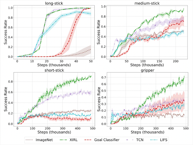
Highlights In our first set of experiments, we checked whether our learned embodiment-invariant reward function can enable successful reinforcement learning, when the expert demonstrations are provided through the agent itself. We find that XIRL significantly outperforms alternative methods especially on the tougher agents (e.g., short-stick and gripper).
Same-embodiment setting: Comparison of XIRL with baseline reward functions, using SAC for RL policy learning. XIRL is roughly 2 to 4 times more sample efficient than some of the baselines on the harder agents (short-stick and gripper).
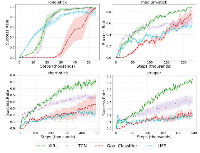
We also find that our approach shows great potential for learning reward functions that generalize to novel embodiments. For instance, when reward learning is performed on embodiments that are different from the ones on which the policy is trained, we find that it results in significantly more sample efficient agents compared to the same baselines. Below, in the gripper subplot (bottom right) for example, the reward is first learned on demonstration videos from long-stick, medium-stick and short-stick, after which the reward function is used to train the gripper agent.
Cross-embodiment setting: XIRL performs favorably when compared with other baseline reward functions, trained on observation-only demonstrations from different embodiments. Each agent (long-stick, medium-stick, short-stick, gripper) had its reward trained using demonstrations from the other three embodiments.
We also find that we can train on real-world human demonstrations, and use the learned reward to train a Sawyer arm in simulation to push a puck to a designated target zone. In these experiments as well, our method outperforms baseline alternatives. For example, our XIRL variant trained only on the real-world demonstrations (purple in the plots below) reaches 80% of the total performance roughly 85% faster than the RLV baseline (orange).
What Do The Learned Reward Functions Look Like? To further explore the qualitative nature of our learned rewards in more challenging real-world scenarios, we collect a dataset of the pen transfer task using various household tools.
Below, we show rewards extracted from a successful (top) and unsuccessful (bottom) demonstration. Both demonstrations follow a similar trajectory at the start of the task execution. The successful one nets a high reward for placing the pens consecutively into the mug then into the glass cup, while the unsuccessful one obtains a low reward because it drops the pens outside the glass cup towards the end of the execution (orange circle). These results are promising because they show that our learned encoder can represent fine-grained visual differences relevant to a task.
Conclusion We highlighted XIRL, our approach to tackling the cross-embodiment imitation problem. XIRL learns an embodiment-invariant reward function that encodes task progress using a temporal cycle-consistency objective. Policies learned using our reward functions are significantly more sample-efficient than baseline alternatives. Furthermore, the reward functions do not require manually paired video frames between the demonstrator and the learner, giving them the ability to scale to an arbitrary number of embodiments or experts with varying skill levels. Overall, we are excited about this direction of work, and hope that our benchmark promotes further research in this area. For more details, please check out our paper and download the code from our GitHub repository.
Acknowledgments Kevin and Andy summarized research performed together with Pete Florence, Jonathan Tompson, Jeannette Bohg (faculty at Stanford University) and Debidatta Dwibedi. All authors would additionally like to thank Alex Nichol, Nick Hynes, Sean Kirmani, Brent Yi, Jimmy Wu, Karl Schmeckpeper and Minttu Alakuijala for fruitful technical discussions, and Sam Toyer for invaluable help with setting up the simulated benchmark.
import os os.environ['TF_CPP_MIN_LOG_LEVEL'] = '2' import tensorflow as tf from tensorflow import keras from tensorflow.keras import layers from tensorflow.keras.datasets import cifar10 tf.__version__ # outputs -> '2.8.0' # Normalizing the data (x_train, y_train), (x_test, y_test) = cifar10.load_data() x_train = x_train.astype("float32") / 255.0 x_test = x_test.astype("float32") / 255.0 # defining Model using Functional api def my_model(): inputs = keras.Input(shape=(32,32,3)) x = layers.Conv2D(32,3)(inputs) x = layers.BatchNormalization()(x) x = keras.activations.relu(x) x = layers.MaxPooling2D()(x) x = layers.Conv2D(64,5,padding="same")(x) x = layers.BatchNormalization()(x) x = keras.activations.relu(x) x = layers.Conv2D(128,3)(x) x = layers.BatchNormalization()(x) x = keras.activations.relu(x) x = layers.Flatten()(x) x = layers.Dense(64, activation='relu')(x) outputs = layers.Dense(10)(x) model = keras.Model(inputs= inputs, outputs=outputs) return model # Building the model model = my_model() # Compiling the model model.compile( loss=keras.losses.SparseCategoricalCrossentropy(from_logits = True), optimizer = keras.optimizers.Adam(learning_rate=3e-4), metrics=['accuracy'], ) # running the model model.fit(x_train, y_train, batch_size= 64, epochs=10, verbose =2) # testing the model model.evaluate(x_test, y_test, batch_size = 1, verbose =2)
I tried this above code on both Jupyter notebook & VSCODE.
On both occasions, its killing the python kernel. Below is the error message screen shot from VS code.
when i run a simple MLP & also deep MLP on MNIST digit dataset. it works fine even when i had more than 10 million parameters. So I am guessing its definitely not the VRAM because for the above CNN model parameters from model.summary( ) = ~400K.
This problem occurs only when i use Conv2D function.
Posted by Sheng Li, Staff Software Engineer and Norman P. Jouppi, Google Fellow, Google Research
Continuing advances in the design and implementation of datacenter (DC) accelerators for machine learning (ML), such as TPUs and GPUs, have been critical for powering modern ML models and applications at scale. These improved accelerators exhibit peak performance (e.g., FLOPs) that is orders of magnitude better than traditional computing systems. However, there is a fast-widening gap between the available peak performance offered by state-of-the-art hardware and the actual achieved performance when ML models run on that hardware.
One approach to address this gap is to design hardware-specific ML models that optimize both performance (e.g., throughput and latency) and model quality. Recent applications of neural architecture search (NAS), an emerging paradigm to automate the design of ML model architectures, have employed a platform-aware multi-objective approach that includes a hardware performance objective. While this approach has yielded improved model performance in practice, the details of the underlying hardware architecture are opaque to the model. As a result, there is untapped potential to build full capability hardware-friendly ML model architectures, with hardware-specific optimizations, for powerful DC ML accelerators.
In “Searching for Fast Model Families on Datacenter Accelerators”, published at CVPR 2021, we advanced the state of the art of hardware-aware NAS by automatically adapting model architectures to the hardware on which they will be executed. The approach we propose finds optimized families of models for which additional hardware performance gains cannot be achieved without loss in model quality (called Pareto optimization). To accomplish this, we infuse a deep understanding of hardware architecture into the design of the NAS search space for discovery of both single models and model families. We provide quantitative analysis of the performance gap between hardware and traditional model architectures and demonstrate the advantages of using true hardware performance (i.e., throughput and latency), instead of the performance proxy (FLOPs), as the performance optimization objective. Leveraging this advanced hardware-aware NAS and building upon the EfficientNet architecture, we developed a family of models, called EfficientNetX, that demonstrate the effectiveness of this approach for Pareto-optimized ML models on TPUs and GPUs.
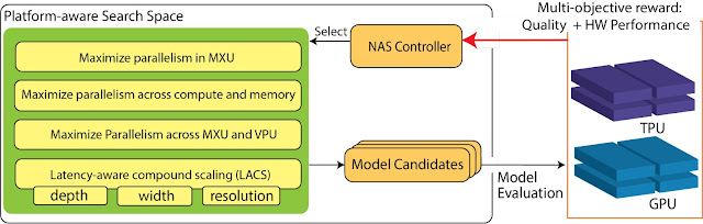
Platform-Aware NAS for DC ML Accelerators To achieve high performance, ML models need to adapt to modern ML accelerators. Platform-aware NAS integrates knowledge of the hardware accelerator properties into all three pillars of NAS: (i) the search objectives; (ii) the search space; and (iii) the search algorithm (shown below). We focus on the new search space because it contains the building blocks needed to compose the models and is the key link between the ML model architectures and accelerator hardware architectures.
We construct TPU/GPU specialized search spaces with TPU/GPU-friendly operations to infuse hardware awareness into NAS. For example, a key adaptation is maximizing parallelism to ensure different hardware components inside the accelerators work together as efficiently as possible. This includes the matrix multiplication units (MXUs) in TPUs and the TensorCore in GPUs for matrix/tensor computation, as well as the vector processing units (VPUs) in TPUs and CUDA cores in GPUs for vector processing. Maximizing model arithmetic intensity (i.e., optimizing the parallelism between computation and operations on the high bandwidth memory) is also critical to achieve top performance. To tap into the full potential of the hardware, it is crucial for ML models to achieve high parallelism inside and across these hardware components.
Overview of platform-aware NAS on TPUs/GPUs, highlighting the search space and search objectives.
Advanced platform-aware NAS has an optimized search space containing a set of complementary techniques to holistically improve parallelism for ML model execution on TPUs and GPUs:
It dynamically selects different activation functions depending on matrix operation types to ensure overlapping of vector and matrix/tensor processing.
It employs hybrid convolutions and a novel fusion strategy to strike a balance between total compute and arithmetic intensity to ensure that computation and memory access happens in parallel and to reduce the contention on VPUs / CUDA cores.
With latency-aware compound scaling (LACS), which uses hardware performance instead of FLOPs as the performance objective to search for model depth, width and resolutions, we ensure parallelism at all levels for the entire model family on the Pareto-front.
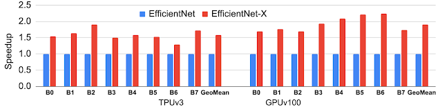
EfficientNet-X: Platform-Aware NAS-Optimized Computer Vision Models for TPUs and GPUs Using this approach to platform-aware NAS, we have designed EfficientNet-X, an optimized computer vision model family for TPUs and GPUs. This family builds upon the EfficientNet architecture, which itself was originally designed by traditional multi-objective NAS without true hardware-awareness as the baseline. The resulting EfficientNet-X model family achieves an average speedup of ~1.5x–2x over EfficientNet on TPUv3 and GPUv100, respectively, with comparable accuracy.
In addition to the improved speeds, EfficientNet-X has shed light on the non-proportionality between FLOPs and true performance. Many think FLOPs are a good ML performance proxy (i.e., FLOPs and performance are proportional), but they are not. While FLOPs are a good performance proxy for simple hardware such as scalar machines, they can exhibit a margin of error of up to 400% on advanced matrix/tensor machines. For example, because of its hardware-friendly model architecture, EfficientNet-X requires ~2x more FLOPs than EfficientNet, but is ~2x faster on TPUs and GPUs.
EfficientNet-X family achieves 1.5x–2x speedup on average over the state-of-the-art EfficientNet family, with comparable accuracy on TPUv3 and GPUv100.
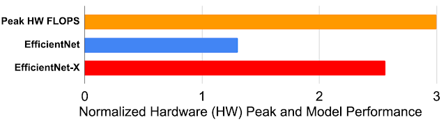
Self-Driving ML Model Performance on New Accelerator Hardware Platforms Platform-aware NAS exposes the inner workings of the hardware and leverages these properties when designing hardware-optimized ML models. In a sense, the “platform-awareness” of the model is a “gene” that preserves knowledge of how to optimize performance for a hardware family, even on new generations, without the need to redesign the models. For example, TPUv4i delivers up to 3x higher peak performance (FLOPS) than its predecessor TPUv2, but EfficientNet performance only improves by 30% when migrating from TPUv2 to TPUv4i. In comparison, EfficientNet-X retains its platform-aware properties even on new hardware and achieves a 2.6x speedup when migrating from TPUv2 to TPUv4i, utilizing almost all of the 3x peak performance gain expected when upgrading between the two generations.
Hardware peak performance ratio of TPUv2 to TPUv4i and the geometric mean speedup of EfficientNet-X and EfficientNet families, respectively, when migrating from TPUv2 to TPUv4i.
Conclusion and Future Work We demonstrate how to improve the capabilities of platform-aware NAS for datacenter ML accelerators, especially TPUs and GPUs. Both platform-aware NAS and the EfficientNet-X model family have been deployed in production and materialize up to ~40% efficiency gains and significant quality improvements for various internal computer vision projects across Google. Additionally, because of its deep understanding of accelerator hardware architecture, platform-aware NAS was able to identify critical performance bottlenecks on TPUv2-v4i architectures and has enabled design enhancements to future TPUs with significant potential performance uplift. As next steps, we are working on expanding platform-aware NAS’s capabilities to the ML hardware and model design beyond computer vision.
Acknowledgements Special thanks to our co-authors: Mingxing Tan, Ruoming Pang, Andrew Li, Liqun Cheng, Quoc Le. We also thank many collaborators including Jeff Dean, David Patterson, Shengqi Zhu, Yun Ni, Gang Wu, Tao Chen, Xin Li, Yuan Qi, Amit Sabne, Shahab Kamali, and many others from the broad Google research and engineering teams who helped on the research and the subsequent broad production deployment of platform-aware NAS.


 Read on how gradient descent and backpropagation algorithms relate to machine learning algorithms.
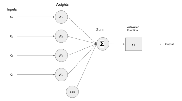


 -> Running this function kills the Python Kernel")