Innovative technologies in AI, virtual worlds and digital humans are shaping the future of design and content creation across every industry. Experience the latest advances from NVIDIA in all these areas at SIGGRAPH, the world’s largest gathering of computer graphics experts, running Aug. 8-11. At the conference, creators, developers, engineers, researchers and students will see Read article >
Posted by Bingyi Cao, Software Engineer, Google Research, and Mário Lipovský, Software Engineer, Google Lens
Computer vision models see daily application for a wide variety of tasks, ranging from object recognition to image-based 3D object reconstruction. One challenging type of computer vision problem is instance-level recognition (ILR) — given an image of an object, the task is to not only determine the generic category of an object (e.g., an arch), but also the specific instance of the object (”Arc de Triomphe de l’Étoile, Paris, France”).
Previously, ILR was tackled using deep learning approaches. First, a large set of images was collected. Then a deep model was trained to embed each image into a high-dimensional space where similar images have similar representations. Finally, the representation was used to solve the ILR tasks related to classification (e.g., with a shallow classifier trained on top of the embedding) or retrieval (e.g., with a nearest neighbor search in the embedding space).
Since there are many different object domains in the world, e.g., landmarks, products, or artworks, capturing all of them in a single dataset and training a model that can distinguish between them is quite a challenging task. To decrease the complexity of the problem to a manageable level, the focus of research so far has been to solve ILR for a single domain at a time. To advance the research in this area, we hosted multiple Kaggle competitions focused on the recognition and retrieval of landmark images. In 2020, Amazon joined the effort and we moved beyond the landmark domain and expanded to the domains of artwork and product instance recognition. The next step is to generalize the ILR task to multiple domains.
To this end, we’re excited to announce the Google Universal Image Embedding Challenge, hosted by Kaggle in collaboration with Google Research and Google Lens. In this challenge, we ask participants to build a single universal image embedding model capable of representing objects from multiple domains at the instance level. We believe that this is the key for real-world visual search applications, such as augmenting cultural exhibits in a museum, organizing photo collections, visual commerce and more.
Images1 of object instances coming from multiple domains, which are represented in our dataset: apparel and accessories, packaged goods, furniture and home goods, toys, cars, landmarks, storefronts, dishes, artwork, memes and illustrations.
Degrees of Variation in Different Domains To represent objects from a large number of domains, we require one model to learn many domain-specific subtasks (e.g., filtering different kinds of noise or focusing on a specific detail), which can only be learned from a semantically and visually diverse collection of images. Addressing each degree of variation proposes a new challenge for both image collection and model training.
The first sort of variation comes from the fact that while some domains contain unique objects in the world (landmarks, artwork, etc.), others contain objects that may have many copies (clothing, furniture, packaged goods, food, etc.). Because a landmark is always placed at the same location, the surrounding context may be useful for recognition. In contrast, a product, say a phone, even of a specific model and color, may have millions of physical instances and thus appear in many surrounding contexts.
Another challenge comes from the fact that a single object may appear different depending on the point of view, lighting conditions, occlusion or deformations (e.g., a dress worn on a person may look very different than on a hanger). In order for a model to learn invariance to all of these visual modes, all of them should be captured by the training data.
Additionally, similarities between objects differ across domains. For example, in order for a representation to be useful in the product domain, it must be able to distinguish very fine-grained details between similarly looking products belonging to two different brands. In the domain of food, however, the same dish (e.g., spaghetti bolognese) cooked by two chefs may look quite different, but the ability of the model to distinguish spaghetti bolognese from other dishes may be sufficient for the model to be useful. Additionally, a vision model of high quality should assign similar representations to more visually similar renditions of a dish.
Which physical objects belong to the instance class?
Single instance in the world
Many physical instances; may differ in size or pattern (e.g., a patterned cloth cut differently)
What are the possible views of the object?
Appearance variation only based on capture conditions (e.g., illumination or viewpoint); limited number of common external views; possibility of many internal views
Deformable appearance (e.g., worn or not); limited number of common views: front, back, side
What are the surroundings and are they useful for recognition?
Surrounding context does not vary much other than daily and yearly cycles; may be useful for verifying the object of interest
Surrounding context can change dramatically due to difference in environment, additional pieces of clothing, or accessories partially occluding clothing of interest (e.g., a jacket or a scarf)
What may be tricky cases that do not belong to the instance class?
Replicas of landmarks (e.g., Eiffel Tower in Las Vegas), souvenirs
Same piece of apparel of different material or different color; visually very similar pieces with a small distinguishing detail (e.g., a small brand logo); different pieces of apparel worn by the same model
Variation among domains for landmark and apparel examples.
Learning Multi-domain Representations After a collection of images covering a variety of domains is created, the next challenge is to train a single, universal model. Some features and tasks, such as representing color, are useful across many domains, and thus adding training data from any domain will likely help the model improve at distinguishing colors. Other features may be more specific to selected domains, thus adding more training data from other domains may deteriorate the model’s performance. For example, while for 2D artwork it may be very useful for the model to learn to find near duplicates, this may deteriorate the performance on clothing, where deformed and occluded instances need to be recognized.
The large variety of possible input objects and tasks that need to be learned require novel approaches for selecting, augmenting, cleaning and weighing the training data. New approaches for model training and tuning, and even novel architectures may be required.
Universal Image Embedding Challenge To help motivate the research community to address these challenges, we are hosting the Google Universal Image Embedding Challenge. The challenge was launched on Kaggle in July and will be open until October, with cash prizes totaling $50k. The winning teams will be invited to present their methods at the Instance-Level Recognition workshop at ECCV 2022.
Participants will be evaluated on a retrieval task on a dataset of ~5,000 test query images and ~200,000 index images, from which similar images are retrieved. In contrast to ImageNet, which includes categorical labels, the images in this dataset are labeled at the instance level.
The evaluation data for the challenge is composed of images from the following domains: apparel and accessories, packaged goods, furniture and home goods, toys, cars, landmarks, storefronts, dishes, artwork, memes and illustrations.
Acknowledgement The core contributors to this project are Andre Araujo, Boris Bluntschli, Bingyi Cao, Kaifeng Chen, Mário Lipovský, Grzegorz Makosa, Mojtaba Seyedhosseini and Pelin Dogan Schönberger. We would like to thank Sohier Dane, Will Cukierski and Maggie Demkin for their help organizing the Kaggle challenge, as well as our ECCV workshop co-organizers Tobias Weyand, Bohyung Han, Shih-Fu Chang, Ondrej Chum, Torsten Sattler, Giorgos Tolias, Xu Zhang, Noa Garcia, Guangxing Han, Pradeep Natarajan and Sanqiang Zhao. Furthermore we are thankful to Igor Bonaci, Tom Duerig, Vittorio Ferrari, Victor Gomes, Futang Peng and Howard Zhou who gave us feedback, ideas and support at various points of this project.
Pinterest has engineered a way to serve its photo-sharing community more of the images they love. The social-image service, with more than 400 million monthly active users, has trained bigger recommender models for improved accuracy at predicting people’s interests. Pinterest handles hundreds of millions of user requests an hour on any given day. And it Read article >
Imagine hiking to a lake on a summer day — sitting under a shady tree and watching the water gleam under the sun. In this scene, the differences between light and shadow are examples of direct and indirect lighting. The sun shines onto the lake and the trees, making the water look like it’s shimmering Read article >
It’s the first GFN Thursday of the month and you know the drill — GeForce NOW is bringing a big batch of games to the cloud. Get ready for 38 exciting titles like Saints Row and Rumbleverse arriving on the GeForce NOW library in August. Members can kick off the month streaming 13 new games Read article >
Posted by Qifei Wang, Senior Software Engineer, and Feng Yang, Senior Staff Software Engineer, Google Research
Deep learning models for visual tasks (e.g., image classification) are usually trained end-to-end with data from a single visual domain (e.g., natural images or computer generated images). Typically, an application that completes visual tasks for multiple domains would need to build multiple models for each individual domain, train them independently (meaning no data is shared between domains), and then at inference time each model would process domain-specific input data. However, early layers between these models generate similar features, even for different domains, so it can be more efficient — decreasing latency and power consumption, lower memory overhead to store parameters of each model — to jointly train multiple domains, an approach referred to as multi-domain learning (MDL). Moreover, an MDL model can also outperform single domain models due to positive knowledge transfer, which is when additional training on one domain actually improves performance for another. The opposite, negative knowledge transfer, can also occur, depending on the approach and specific combination of domains involved. While previous work on MDL has proven the effectiveness of jointly learning tasks across multiple domains, it involved a hand-crafted model architecture that is inefficient to apply to other work.
In “Multi-path Neural Networks for On-device Multi-domain Visual Classification”, we propose a general MDL model that can: 1) achieve high accuracy efficiently (keeping the number of parameters and FLOPS low), 2) learn to enhance positive knowledge transfer while mitigating negative transfer, and 3) effectively optimize the joint model while handling various domain-specific difficulties. As such, we propose a multi-path neural architecture search (MPNAS) approach to build a unified model with heterogeneous network architecture for multiple domains. MPNAS extends the efficient neural architecture search (NAS) approach from single path search to multi-path search by finding an optimal path for each domain jointly. Also, we introduce a new loss function, called adaptive balanced domain prioritization (ABDP) that adapts to domain-specific difficulties to help train the model efficiently. The resulting MPNAS approach is efficient and scalable; the resulting model maintains performance while reducing the model size and FLOPS by 78% and 32%, respectively, compared to a single-domain approach.
Multi-Path Neural Architecture Search To encourage positive knowledge transfer and avoid negative transfer, traditional solutions build an MDL model so that domains share most of the layers that learn the shared features across domains (called feature extraction), then have a few domain-specific layers on top. However, such a homogenous approach to feature extraction cannot handle domains with significantly different features (e.g., objects in natural images and art paintings). On the other hand, handcrafting a unified heterogeneous architecture for each MDL model is time-consuming and requires domain-specific knowledge.
NAS is a powerful paradigm for automatically designing deep learning architectures. It defines a search space, made up of various potential building blocks that could be part of the final model. The search algorithm finds the best candidate architecture from the search space that optimizes the model objectives, e.g., classification accuracy. Recent NAS approaches (e.g., TuNAS) have meaningfully improved search efficiency by using end-to-end path sampling, which enables us to scale NAS from single domains to MDL.
Inspired by TuNAS, MPNAS builds the MDL model architecture in two stages: search and training. In the search stage, to find an optimal path for each domain jointly, MPNAS creates an individual reinforcement learning (RL) controller for each domain, which samples an end-to-end path (from input layer to output layer) from the supernetwork (i.e., the superset of all the possible subnetworks between the candidate nodes defined by the search space). Over multiple iterations, all the RL controllers update the path to optimize the RL rewards across all domains. At the end of the search stage, we obtain a subnetwork for each domain. Finally, all the subnetworks are combined to build a heterogeneous architecture for the MDL model, shown below.
Since the subnetwork for each domain is searched independently, the building block in each layer can be shared by multiple domains (i.e., dark gray nodes), used by a single domain (i.e., light gray nodes), or not used by any subnetwork (i.e., dotted nodes). The path for each domain can also skip any layer during search. Given the subnetwork can freely select which blocks to use along the path in a way that optimizes performance (rather than, e.g., arbitrarily designating which layers are homogenous and which are domain-specific), the output network is both heterogeneous and efficient.
Example architecture searched by MPNAS. Dashed paths represent all the possible subnetworks. Solid paths represent the selected subnetworks for each domain (highlighted in different colors). Nodes in each layer represent the candidate building blocks defined by the search space.
The figure below demonstrates the searched architecture of two visual domains among the ten domains of the Visual Domain Decathlon challenge. One can see that the subnetwork of these two highly related domains (one red, the other green) share a majority of building blocks from their overlapping paths, but there are still some differences.
Architecture blocks of two domains (ImageNet and Describable Textures) among the ten domains of the Visual Domain Decathlon challenge. Red and green path represents the subnetwork of ImageNet and Describable Textures, respectively. Dark pink nodes represent the blocks shared by multiple domains. Light pink nodes represent the blocks used by each path. The model is built based on MobileNet V3-like search space. The “dwb” block in the figure represents the dwbottleneck block. The “zero” block in the figure indicates the subnetwork skips that block.
Below we show the path similarity between domains among the ten domains of the Visual Domain Decathlon challenge. The similarity is measured by the Jaccard similarity score between the subnetworks of each domain, where higher means the paths are more similar. As one might expect, domains that are more similar share more nodes in the paths generated by MPNAS, which is also a signal of strong positive knowledge transfer. For example, the paths for similar domains (like ImageNet, CIFAR-100, and VGG Flower, which all include objects in natural images) have high scores, while the paths for dissimilar domains (like Daimler Pedestrian Classification and UCF101 Dynamic Images, which include pedestrians in grayscale images and human activity in natural color images, respectively) have low scores.
Confusion matrix for the Jaccard similarity score between the paths for the ten domains. Score value ranges from 0 to 1. A greater value indicates two paths share more nodes.
Training a Heterogeneous Multi-domain Model In the second stage, the model resulting from MPNAS is trained from scratch for all domains. For this to work, it is necessary to define a unified objective function for all the domains. To successfully handle a large variety of domains, we designed an algorithm that adapts throughout the learning process such that losses are balanced across domains, called adaptive balanced domain prioritization (ABDP).
Below we show the accuracy, model size, and FLOPS of the model trained in different settings. We compare MPNAS to three other approaches:
Domain independent NAS: Searching and training a model for each domain separately.
Single path multi-head: Using a pre-trained model as a shared backbone for all domains with separated classification heads for each domain.
Multi-head NAS: Searching a unified backbone architecture for all domains with separated classification heads for each domain.
From the results, we can observe that domain independent NAS requires building a bundle of models for each domain, resulting in a large model size. Although single path multi-head and multi-head NAS can reduce the model size and FLOPS significantly, forcing the domains to share the same backbone introduces negative knowledge transfer, decreasing overall accuracy.
Model
Number of parameters ratio
GFLOPS
Average Top-1 accuracy
Domain independent NAS
5.7x
1.08
69.9
Single path multi-head
1.0x
0.09
35.2
Multi-head NAS
0.7x
0.04
45.2
MPNAS
1.3x
0.73
71.8
Number of parameters, gigaFLOPS, and Top-1 accuracy (%) of MDL models on the Visual Decathlon dataset. All methods are built based on the MobileNetV3-like search space.
MPNAS can build a small and efficient model while still maintaining high overall accuracy. The average accuracy of MPNAS is even 1.9% higher than the domain independent NAS approach since the model enables positive knowledge transfer. The figure below compares per domain top-1 accuracy of these approaches.
Top-1 accuracy of each Visual Decathlon domain.
Our evaluation shows that top-1 accuracy is improved from 69.96% to 71.78% (delta: +1.81%) by using ABDP as part of the search and training stages.
Top-1 accuracy for each Visual Decathlon domain trained by MPNAS with and without ABDP.
Future Work We find MPNAS is an efficient solution to build a heterogeneous network to address the data imbalance, domain diversity, negative transfer, domain scalability, and large search space of possible parameter sharing strategies in MDL. By using a MobileNet-like search space, the resulting model is also mobile friendly. We are continuing to extend MPNAS for multi-task learning for tasks that are not compatible with existing search algorithms and hope others might use MPNAS to build a unified multi-domain model.
Acknowledgements This work is made possible through a collaboration spanning several teams across Google. We’d like to acknowledge contributions from Junjie Ke, Joshua Greaves, Grace Chu, Ramin Mehran, Gabriel Bender, Xuhui Jia, Brendan Jou, Yukun Zhu, Luciano Sbaiz, Alec Go, Andrew Howard, Jeff Gilbert, Peyman Milanfar, and Ming-Tsuan Yang.
Starting today, the NVIDIA Jetson AGX Orin 32GB production module is available for purchase. Combined with the world-standard NVIDIA AI software stack and an…
Starting today, the NVIDIA Jetson AGX Orin 32GB production module is available for purchase. Combined with the world-standard NVIDIA AI software stack and an ecosystem of services and products, the road to market has never been faster.
The NVIDIA Jetson AGX Orin 32GB module delivers up to 200 trillion operations per second (TOPS) of AI performance with power configurable between 15W and 40W, which is more than 6x the performance of Jetson AGX Xavier in the same compact form-factor for robotics and other autonomous machine use cases.
This latest system-on-module supports multiple concurrent AI application pipelines with an NVIDIA Ampere architecture GPU, next-generation deep learning and vision accelerators, high-speed IO, and fast memory bandwidth. Developers can build solutions using their largest and most complex AI models to solve problems such as natural language understanding, 3D perception, and multi-sensor fusion.
Jetson runs the NVIDIA AI software stack, and use-case specific application frameworks are available, including NVIDIA Isaac for robotics, DeepStream for vision AI, and Riva for conversational AI.
You can also save time using the NVIDIA Omniverse Replicator for synthetic data generation (SDG), and with NVIDIA TAO Toolkit for fine-tuning pretrained AI models from the NGC catalog.
A broad range of Jetson ecosystem partners offer additional AI and system software, developer tools, and custom software development. They can also help with cameras and other sensors, as well as full system carrier boards and design services for your product.
Learn more about all the partners solutions supporting Orin that were announced today.
The Jetson AGX Orin Developer Kit is also available now. Use it to accelerate your Orin development, emulate the entire family of Jetson Orin modules, and create advanced robotics and edge AI applications.
Look for additional Jetson Orin modules later this year, including Jetson Orin NX 16GB in October, Jetson AGX Orin 64GB in November, and Jetson Orin NX 8GB in December. Sign up to be notified when new Jetson Orin modules become available.
This is the first part of a two-part series discussing the NVIDIA FasterTransformer library, one of the fastest libraries for distributed inference of…
This is the first part of a two-part series discussing the NVIDIA FasterTransformer library, one of the fastest libraries for distributed inference of transformers of any size (up to trillions of parameters). It provides an overview of FasterTransformer, including the benefits of using the library.
Transformers are among the most influential AI model architectures today and are shaping the direction for future R&D in AI. Invented first as a tool for natural language processing (NLP), they are now used for almost any AI task, including computer vision, automatic speech recognition, classification of molecule structures, and processing of financial data. Accounting for such widespread use is the attention mechanism, which noticeably increases the computational efficiency, quality, and accuracy of the models.
Large transformer-based models with hundreds of billions of parameters behave like a gigantic encyclopedia and brain that contains information about everything it has learned. They structurize, represent, and summarize all this knowledge in a unique way. Having such models with this vast amount of prior knowledge allows us to use new and powerful one-shot or few-shot learning techniques to solve many NLP tasks.
Thanks to their computational efficiency, transformers scale well–and by increasing the size of the network and the amount of training data, researchers can improve observations and increase accuracy.
Training such large models is a non-trivial task, however. The models may require more memory than one GPU supplies–or even hundreds of GPUs. Thankfully, NVIDIA researchers have created powerful open-source tools, such as NeMo Megatron, that optimize the training process.
Fast and optimized inference allows enterprises to realize the full potential of these large models. The latest research demonstrates that increasing the size of the model as well as the dataset increases the quality of such a model on downstream tasks in different domains (NLP, CV, and others).
At the same time, data show that such a technique also works in multi-domain tasks. (See research papers like OpenAI’s DALLE-2 and Google’s Imagen on text-to-image generation, for example.) Research directions such as p-tuning that rely on “frozen” copies of huge models even increase the importance of having a stable and optimized inference pipeline. Optimized inference of such large models requires distributed multi-GPU multi-node solutions.
A library for accelerated inference of large transformers
NVIDIA FasterTransformer (FT) is a library implementing an accelerated engine for the inference of transformer-based neural networks, with a special emphasis on large models, spanning many GPUs and nodes in a distributed manner.
FasterTransformer contains the implementation of the highly-optimized version of the transformer block that contains the encoder and decoder parts.
Using this block, you can run the inference of both the full encoder-decoder architectures like T5, as well as encoder-only models, such as BERT, or decoder-only models, such as GPT. It is written in C++/CUDA and relies on the highly optimized cuBLAS, cuBLASLt , and cuSPARSELt libraries. This allows you to build the fastest transformer inference pipeline on GPU.
Figure 1. A couple of transformer/attention blocks are distributed between four GPUs using tensor parallelism (tensor MP partitions) and pipeline parallelism (pipeline MP partitions)
The distinctive feature of FT in comparison with other compilers like NVIDIA TensorRT is that it supports the inference of large transformer models in a distributed manner.
Figure 1 shows how a neural network with multiple classical transformer/attention layers could be split onto multiple GPUs and nodes using tensor parallelism (TP) and pipeline parallelism (PP) techniques.
Tensor parallelism occurs when each tensor is split up into multiple chunks, and each chunk of the tensor can be placed on a separate GPU. During computation, each chunk gets processed separately in-parallel on different GPUs and the results (final tensor) can be computed by combining results from multiple GPUs.
Pipeline parallelism occurs when a model is split up in-depth and different fulllayers are placed onto different GPUs/nodes.
Under the hood, enabling inter/intra-node communication relies on MPI and NVIDIA NCCL. Using this software stack, you can run large transformers in tensor parallelism mode on multiple GPUs to reduce computational latency.
At the same time, TP and PP may be combined together to run large transformer models with billions and trillions of parameters (which amount to terabytes of weights) on multi-GPU and multi-node environments.
Aside from the source codes in C, FasterTransformer also provides TensorFlow integration (using the TensorFlow op), PyTorch integration (using the PyTorch op), and Triton integration as a backend.
Currently, TensorFlow op only supports a single GPU, while PyTorch op and Triton backend both support multi-GPU and multi-node.
To prevent the additional work of splitting the model for model parallelism, FasterTransformer also provides a tool to split and convert models from different formats to the FasterTransformer binary file format. Then FasterTransformer can load the model in a binary format directly.
At this time, FT supports models like Megatron-LM GPT-3, GPT-J, BERT, ViT, Swin Transformer, Longformer, T5, and XLNet. You can check the latest support matrix in the FasterTransformer repo on GitHub.
FT works on GPUs with compute capability >= 7.0, such as V100, A10, A100, and others.
Figure 2. GPT-J 6B model inference speed-up comparison
Optimizations in FasterTransformer
FT enables you to get a faster inference pipeline, with lower latency and higher throughput for the transformer-based NNs in comparison to the common frameworks for deep learning training.
Some of the optimization techniques that allow FT to have the fastest inference for the GPT-3 and other large transformer models include:
Layer fusion – The set of techniques in the pre-processing stage that combine multiple layers of NNs into a single one that would be computed with one single kernel. This technique reduces data transfer and increases math density, thus accelerating computation at the inference stage. For example, all the operations in the multi-head attention block can be combined into one kernel.
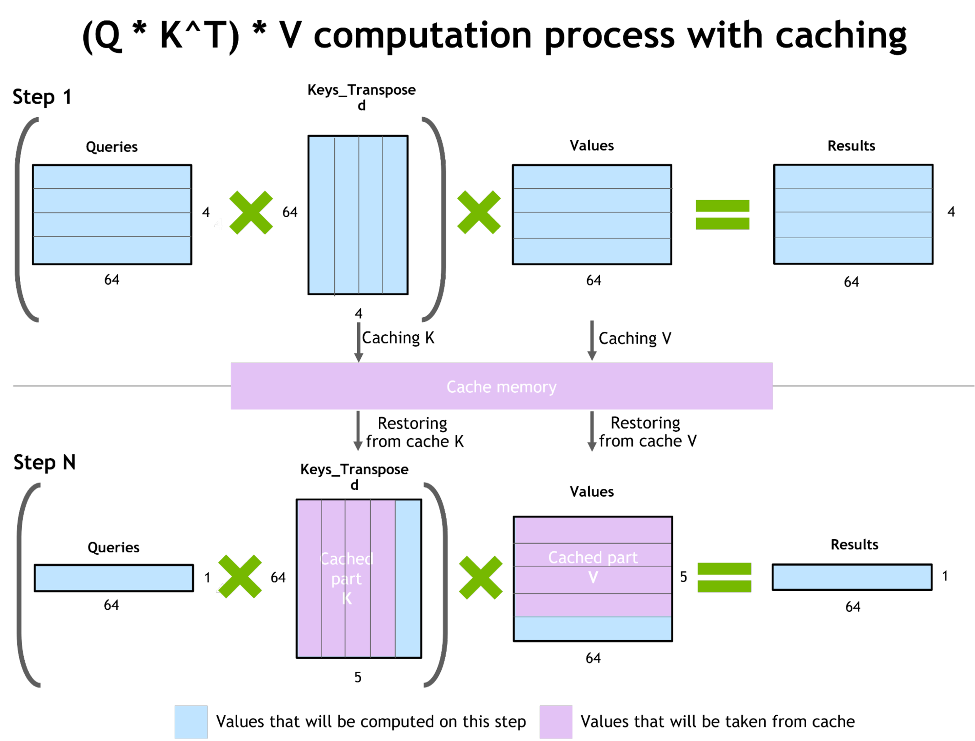
Figure 3. Demonstration of the caching mechanism in the NVIDIA FasterTransformer library
Inference optimization for autoregressive models / activations caching
To prevent recomputing the previous keys and values for each new token generator by transformer, FT allocates a buffer to store them at each step.
Although it takes some additional memory usage, FT can save the cost of recomputing, allocating a buffer at each step, and the cost of concatenation. The scheme of the process is presented in Figure 2. The same caching mechanism is used in multiple parts of the NN.
Memory optimization
Different from traditional models like BERT, large transformer models have up to trillions of parameters taking hundreds of GB of storage. GPT-3 175b takes 350 GB even if we store the model in half-precision. It’s therefore necessary to reduce memory usage for other parts.
For example, in FasterTransformer, we reuse the memory buffer of activations/outputs in different decoder layers. Since the number of layers in GPT-3 is 96, we only need 1/96 of the amount of memoryfor activations.
Usage of MPI and NCCL to enable inter/intra-node communication and support model parallelism
In the GPT model, FasterTransormer provides both tensor parallelism and pipeline parallelism. For tensor parallelism, FasterTransformer follows the idea of Megatron. For both the self-attention block and feed-forward network block, FT split the weights of the first matrix by row and split the weights of the second matrix by column. By optimization, FT can reduce the reduction operation to two times for each transformer block.
For pipeline parallelism, FasterTransformer splits the whole batch of requests into multiple micro-batches, hiding the bubble of communication. FasterTransformer will adjust the micro-batch size automatically for different cases.
MatMul kernel autotuning (GEMM autotuning)
Matrix multiplication is the main and the heaviest operation in transformer-based neural networks. FT uses functionalities from CuBLAS and CuTLASS libraries to execute these types of operations. It is important to know that MatMul operation can be executed in tens of different ways using different low-level algorithms at the “hardware” level.
GemmBatchedEx function implements MatMul operation and has “cublasGemmAlgo_t” as an input parameter. Using this parameter, you can choose different low-level algorithms for operation.
The FasterTransformer library uses this parameter to do a real-time benchmark of all low-level algorithms and to choose the best one for the parameters of the model (size of the attention layers, number of attention heads, size of the hidden layer) and for your input data. Additionally, FT uses hardware-accelerated low-level functions for some parts of the network such as __expf, __shfl_xor_sync.
Inference with lower precisions
FT has kernels that support inference using low-precision input data in fp16 and int8. Both these regimes allow acceleration due to a lower amount of data transfer and required memory. At the same time, int8 and fp16 computations can be executed on special hardware, such as the tensor cores (for all GPU architectures starting from Volta), and the transformers engine in the upcoming Hopper GPUs.
More
Rapidly fast C++ BeamSearch implementation
Optimized all-reduce for the TensorParallelism 8 mode When the weights parts of the model are split between eight GPUs
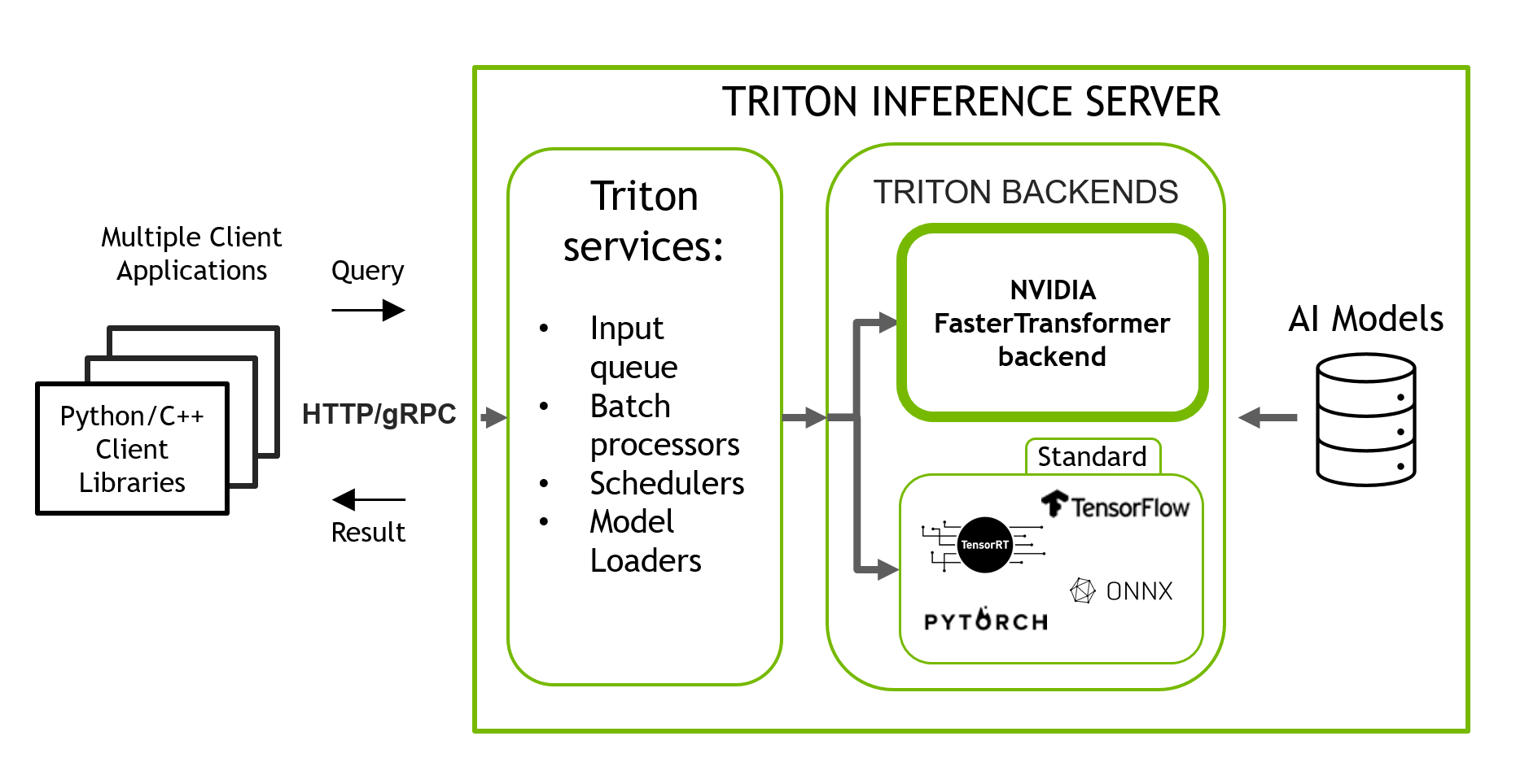
NVIDIA Triton inference server with FasterTransformer backend
NVIDIA Triton Inference Server is an open-source inference serving software that helps standardize model deployment and execution, delivering fast and scalable AI in production. Stable and fast, Triton allows you to run inference of your ML/DL models in a simple manner with a pre-baked Docker container using only one line of code and a simple JSON-like config.
Triton supports models using multiple backends such as PyTorch, TorchScript, Tensorflow, ONNXRuntime, and OpenVINO. Triton takes your exported model that was trained in one of the frameworks and runs this model in inference using the corresponding backend transparently for you. It can also be extended with custom backends. Triton wraps your model with HTTP/gRPC API and provides client-side libraries for multiple languages.
Figure 4. Triton inference server with multiple backends for inference of model trained with different frameworks
Triton includes the FasterTransformer library as a backend (Figure 4) that enables running distributed multi-GPU, multi-node inference of large transformer models with TP and PP. Today, GPT-J, GPT-Megatron, and T5 models are supported in Triton with FasterTransformer backend.
This is the second part of a two-part series about NVIDIA tools that allow you to run large transformer models for accelerated inference. For an introduction to…
This post is a guide to optimized inference of large transformer models such as EleutherAI’s GPT-J 6B and Google’s T5-3B. Both of these models demonstrate good results in many downstream tasks and are among the most available to researchers and data scientists.
NVIDIA FasterTransformer (FT) in NVIDIA Triton allows you to run both of these models in a similar and simple manner while providing enough flexibility to integrate/combine with other inference or training pipelines. The same NVIDIA software stack can be used for inference of the trillion-parameters models combining tensor parallelism (TP) and pipeline parallelism (PP) techniques on multiple nodes.
Transformer models are increasingly used in numerous domains and demonstrate outstanding accuracy. More importantly, the size of the model directly affects its quality. Apart from the NLP, this is applicable to other domains as well.
Researchers from Google demonstrated that the scaling of the transformer-based text encoder was crucial for the whole image generation pipeline in their Imagen model, the latest and one of the most promising generative text-to-image models. Scaling the transformers leads to outstanding results in both single and multi-domain pipelines. This guide uses transformer-based models of the same structure and a similar size.
Overview and walkthrough of main steps
This section presents the main steps for running T5 and GPT-J in optimized inference using FasterTransformer and Triton Inference Server. Figure 1 demonstrates the overall process for one neural network.
It is highly recommended to do all the steps in a Docker container to reproduce the results. Instructions about preparing a FasterTransformer Docker container are available at the beginning of the same notebook.
If you have pretrained one of these models, you will have to convert the weights from your framework saved-model files into the binary format recognizable by the FT. Scripts for conversion are provided in the FasterTransformer repository.
Figure 1. An overall pipeline of the transformer neural network with FasterTransformer and Triton
Steps 1 and 2: Build Docker container with Triton inference server and FasterTransformer backend. Use the Triton inference server as the main serving tool proxying requests to the FasterTransformer backend.
Steps 3 and 4: Build the FasterTransformer library. This library contains many useful tools for inference preparation as well as bindings for multiple languages and examples of how to do inference in C++ and Python.
Steps 5 and 6: Download weights of the pretrained models (T5-3B and GPT-J) and prepare them for the inference with FT by converting into binary format and splitting them into multiple partitions for parallelism and accelerated inference. Code from the FasterTransformer library will be used in this step.
Step 7: Use code from the FasterTransformer library to find optimal low-level kernels for the NN.
Step 8: Start the Triton server that uses all artifacts from previous steps and run the Python client code to send requests to the server with accelerated models.
Step 1: Clone fastertransformer_backend from the Triton GitHub repository
All further steps need to be run inside the Docker container interactive session. Jupyter Lab is also needed in this container to work with the notebook provided.
The Docker container was built with Triton and FasterTransformer and started with the fastertransformer_backend source codes inside.
Steps 3 and 4: Clone FasterTransformer source codes and build the library
The FasterTransformer library is pre-built and placed into our container during the Docker build process.
Download the FasterTransformer source code from GitHub to use the additional scripts that allow converting the pre-trained model files of the GPT-J or T5 into FT binary format that will be used at the time of inference.
GPT-J is a decoder model that was developed by EleutherAI and trained on The Pile, an 825GB dataset curated from multiple sources. With 6 billion parameters, GPT-J is one of the largest GPT-like publicly-released models.
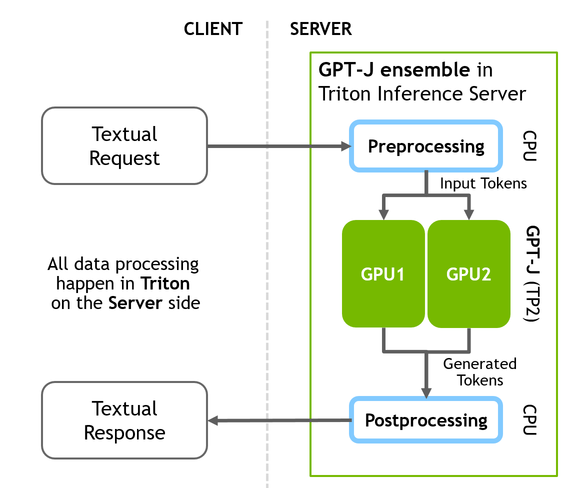
FasterTransformer backend has a config for the GPT-J model under fastertransformer_backend/all_models/gptj. This config is a perfect demonstration of a Triton ensemble. Triton allows you to run a single model inference, as well as construct complex pipes/pipelines comprising many models required for an inference task.
You can also add additional Python/C++ scripts before and/or after any neural network for pre/post processing steps that could transform your data/results into the final form.
The GPT-J inference pipeline includes three different sequential steps at the server side:
The config file combines all three stages into a single pipeline. Figure 2 illustrates the client-server inference scheme.
Figure 2. GPT-J inference with FasterTransformer and Triton. Scheme of the ensemble with all pre- and post-processing steps happening on the server side
Steps 5-8 are the same for both GPT-J and T5 and are provided below (GPT first, followed by T5).
Step 5 (GPT-J): Download and prepare weights of the GPT-J model
wget https://mystic.the-eye.eu/public/AI/GPT-J-6B/step_383500_slim.tar.zstd
tar -axf step_383500_slim.tar.zstd -C ./models/
These weights need to be converted into the binary format recognized by the C++ FasterTransformer backend. FasterTransformer provides the tools/scripts for different pretrained neural networks.
For the GPT-J weights you can use the script:
FasterTransformer/examples/pytorch/gptj/utils/gptj_ckpt_convert.py to convert the checkpoint as follows:
The n-inference-gpus specifies the number of GPUs for tensor parallelism. This script will create ./models/j6b_ckpt/2-gpu directory and automatically write prepared weights there. These weights will be ready for TensorParallel 2 inference. Using this parameter, you can split your weights onto a larger number of GPUs to achieve even higher speed using the TP technique.
Step 7 (GPT-J): Kernel-autotuning for the GPT-J inference
The next step is kernel-autotuning. Matrix multiplication is the main and the heaviest operation in transformer-based neural networks. FT uses functionalities from CuBLAS and CuTLASS libraries to execute this type of operation. It is important to note that MatMul operation can be executed in tens of different ways using different low-level algorithms at the “hardware” level.
The FasterTransformer library has a script that allows real-time benchmarking of all low-level algorithms and selection of the best one for the parameters of the model (size of the attention layers, number of attention heads, size of the hidden layer) and for your input data. This step is optional but achieves a higher inference speed.
Run the ./FasterTransformer/build/bin/gpt_gemm binary file that was built at the stage of building FasterTransformer library. Arguments for the script may be found in the GitHub’s documentation or by using --help argument.
Step 8 (GPT-J): Prepare the Triton config and serve the model
With the weights ready, the next step is to prepare a Triton config file for the GPT-J model. Open the main Triton config for the GPT-J model at fastertransformer_backend/all_models/gptj/fastertransformer/config.pbtxt for editing. Only two mandatory parameters need to be changed there to start inference.
Update tensor_para_size. Weights were prepared for two GPUs, so set it equal to 2.
If Triton starts successfully, you will see output lines informing that the models are loaded by Triton and the server is listening the designated ports for incoming requests:
# Info about T5 model that was found by the Triton in our directory:

+-------------------+---------+--------+
| Model             | Version | Status |
+-------------------+---------+--------+
| fastertransformer | 1       | READY  |
+-------------------+---------+--------+

# Info about that Triton successfully started and waiting for HTTP/GRPC requests:

I0503 17:26:25.226719 1668 grpc_server.cc:4421] Started GRPCInferenceService at 0.0.0.0:8001
I0503 17:26:25.227017 1668 http_server.cc:3113] Started HTTPService at 0.0.0.0:8000
I0503 17:26:25.283046 1668 http_server.cc:178] Started Metrics Service at 0.0.0.0:8002
Next, send the inference requests to the server. On the client side, the tritonclient Python library allows communicating with our server from any of the Python apps.
This example with GPT-J sends textual data straight to the Triton server and all preprocessing and postprocessing will happen on the server side. The full client script can be found at fastertransformer_backend/tools/end_to_end_test.py or in the Jupyter notebook provided.
The main parts include:
# Import libraries
import tritonclient.http as httpclient

# Initizlize client
client = httpclient.InferenceServerClient("localhost:8000",
                                           concurrency=1,
                                           verbose=False)
# ...

# Request text promp from user
print("Write any input prompt for the model and press ENTER:")
# Prepare tokens for sending to the server
inputs = prepare_inputs( [[input()]])
# Sending request
result = client.infer(MODEl_GPTJ_FASTERTRANSFORMER, inputs)
print(result.as_numpy("OUTPUT_0"))
T5 inference
T5 (Text-to-Text Transfer Transformer) is a recent architecture created by Google. It consists of encoder and decoder parts and is an instance of a full transformer architecture. It reframes all the natural language processing (NLP) tasks into a unified text-to-text format where the input and output are always text strings.
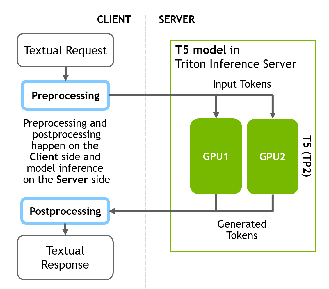
The T5 inference pipeline prepared in this section differs from the GPT-J model, in that only the NN inference stage is on the server side, not a full pipeline with data preprocessing and results in postprocessing. All computations for the pre- and post-processing stages are happening on the client side.
Triton allows you to configure your inference flexibly so it is possible to build a full pipeline on the server side too, but other configurations are also possible.
First, do a conversion from text into tokens in Python using the Huggingface library on the client side. Next, send an inference request to the server. Finally, after getting a response from the server, convert the generated tokens into text on the client side.
Figure 3 illustrates the client-server inference scheme.
Figure 3. T5 inference with FasterTransformer and Triton. All pre- and post-processing steps happen on the client side and only the heavy inference part computes is on the server.
Preparation steps for T5 are the same as for GPT-J. Details for steps 5-8 are provided below for T5:
Step 5 (T5): Download weights of the T5-3B
First download weights of the T5 3b size. You will have to install git-lfs to successfully download the weights.
git clone https://huggingface.co/t5-3b
Step 6 (T5): Convert weights into FT format
Again, the weights need to be converted into the binary format recognized by the C++ FasterTransformer backend. For T5 weights you can use the script at FasterTransformer/blob/main/examples/pytorch/t5/utils/huggingface_t5_ckpt_convert.py to convert the checkpoint.
The converter requires the following arguments. Quite similar to GPT-J but parameter i_g means the number of GPUs will be used for the inference in TP regime, so set it to 2:
Step 7 (T5): Kernel-autotuning for the T5-3B inference
The next step is kernel-autotuning for T5 using the t5_gemm binary file that will run experiments to benchmark the heaviest parts of the T5 model and find the best low-level kernels. Run ./FasterTransformer/build/bin/t5_gemm binary file that was built at the stage of building the FasterTransformer library (Step 2). This step is optional but including it achieves a higher inference speed. Again, the arguments for the script may be found in the GitHub’s documentation or by using --help argument.
Step 8 (T5): Prepare the Triton config of the T5 model
You will have to open the copied Triton config for the T5 model triton-model-store/t5/fastertransformer/config.pbtxt for editing. Only two mandatory parameters need to be changed there to start the inference.
Then update tensor_para_size. Weights were prepared for two GPUs, so set it to 2.
If Triton starts successfully, you will see these lines in the output:
# Info about T5 model that was found by the Triton in our directory:

+-------------------+---------+--------+
| Model             | Version | Status |
+-------------------+---------+--------+
| fastertransformer | 1       | READY  |
+-------------------+---------+--------+

# Info about that Triton successfully started and waiting for HTTP/GRPC requests:

I0503 17:26:25.226719 1668 grpc_server.cc:4421] Started GRPCInferenceService at 0.0.0.0:8001
I0503 17:26:25.227017 1668 http_server.cc:3113] Started HTTPService at 0.0.0.0:8000
I0503 17:26:25.283046 1668 http_server.cc:178] Started Metrics Service at 0.0.0.0:8002
Now run the client script. On the client side, transform the textual input to tokens using the Huggingface library and only then send a request to the server using the Python’s tritonclient library. Implement function preprocessing for this purpose.
Then use an instance of the tritonclient http class that will request the 8000 port on the server (“localhost” if deployed locally) to send tokens to the model through HTTP.
After receiving the response containing the tokens, again transform the tokens into text form using a postprocessing helper function.
# Import libraries
from transformers import (
    T5Tokenizer,
    T5TokenizerFast
)
import tritonclient.http as httpclient

# Initialize client
client = httpclient.InferenceServerClient(
    URL, concurrency=request_parallelism, verbose=verbose
)

# Initialize tokenizers from HuggingFace to do pre and post processings
# (convert text into tokens and backward) at the client side
tokenizer = T5Tokenizer.from_pretrained(MODEL_T5_HUGGINGFACE, model_max_length=1024)
fast_tokenizer = T5TokenizerFast.from_pretrained(MODEL_T5_HUGGINGFACE, model_max_length=1024)

# Implement the function that takes text converts it into the tokens using
# HFtokenizer and prepares tensorts for sending to Triton
def preprocess(t5_task_input):
    ...

# Implement function that takes tokens from Triton's response and converts
# them into text
def postprocess(result):
    ...

# Run translation task with T5
text = "Translate English to German: He swung back the fishing pole and cast the line."
inputs = preprocess(text)
result = client.infer(MODEl_T5_FASTERTRANSFORMER, inputs)
postprocess(result)
Adding custom layers and new NN architectures
If you have some custom neural network with the transformer blocks inside, or you have added some custom layers into default NNs supported by FT (T5, GPT), this NN won’t be supported by FT out-of-the-box. You can either change the source code of FT to add support for this NN by adding support for new layers, or you can use FT blocks and C++, PyTorch, and TensorFlow API to integrate fast transformer blocks from FT into your custom inference script/pipeline.
Results
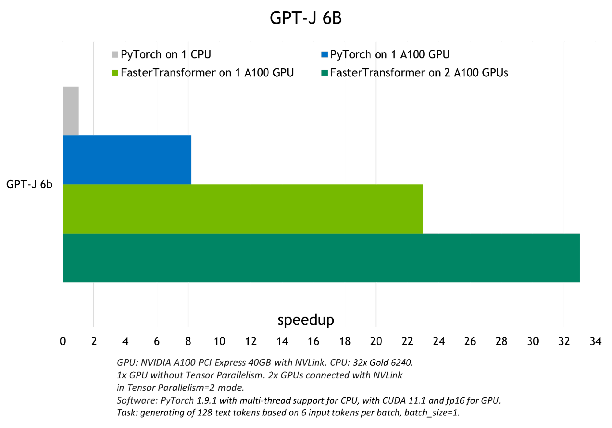
The optimizations carried out by FasterTransformer achieved up to 6xspeed-up over native PyTorch GPU inference in FP16 mode and up to 33x speedup over PyTorch CPU inference for GPT-J and T5-3B.
Figure 4 shows the inference results for the GPT-J, and Figure 5 shows the inference results for T5-3B model at batch size 1 for the translation task.
Figure 4. GPT-J 6B model inference speed-up comparison
Figure 5. T5-3B model inference speed-up comparison
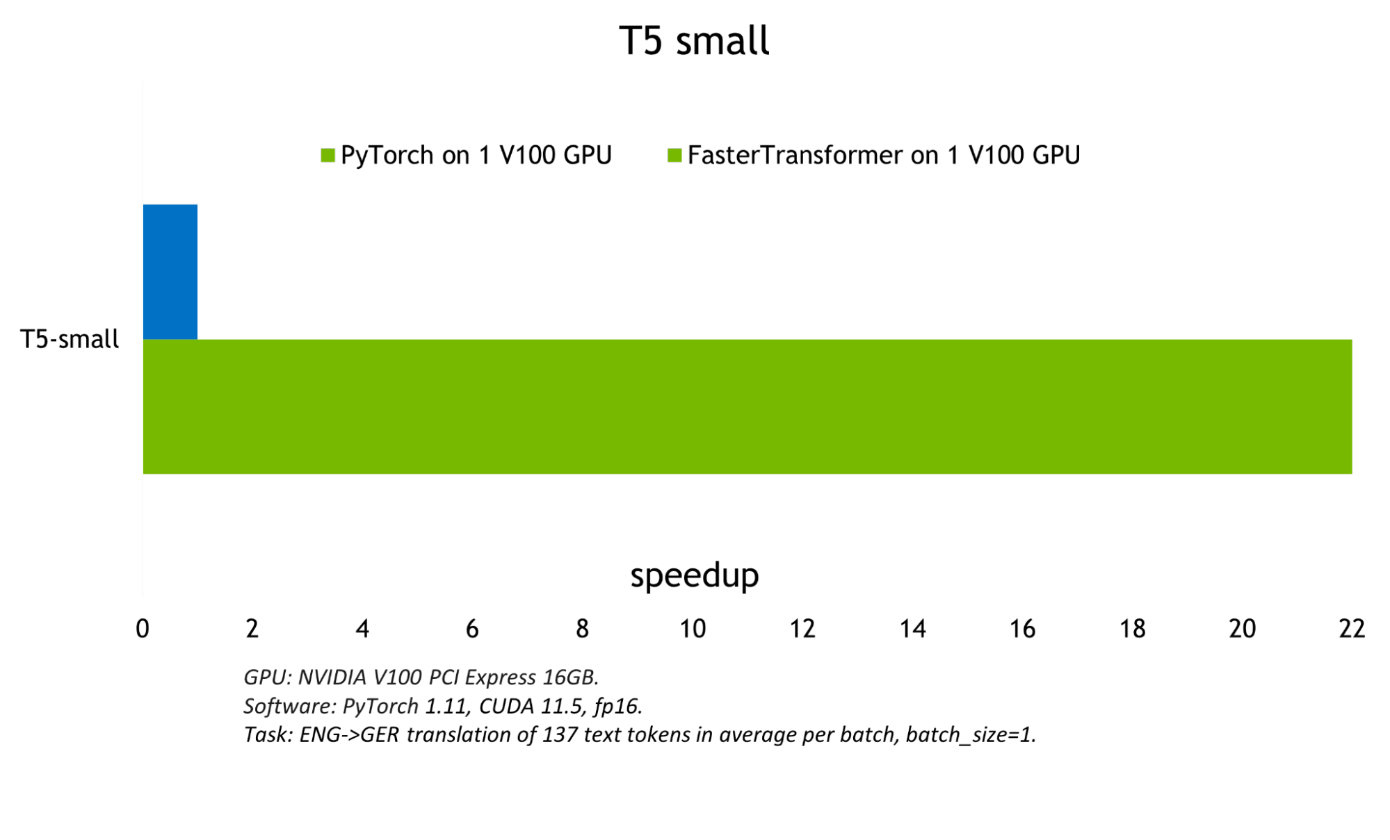
The smaller the model and the bigger the batch size, the better optimization FasterTransformer demonstrates due to increasing computational bandwidth. Figure 6 shows the T5-small model, tests of which can be found on the FasterTrasformer GitHub. It demonstrates a ~22x throughput increase in comparison with GPU PyTorch inference. Similar results can be found on GitHub for the T5-base model.
Figure 6. T5-small model inference comparison
Conclusion
The code example demonstrated here uses FasterTransformer and Triton inference server to run inference of the GPT-J-6B and T5-3B models. It achieved up to 33x acceleration in comparison with CPU and up to 22x in comparison with native PyTorch backend on GPU.
The same approach can be used for small transformer models like T5-small and BERT as well as huge models with trillions of parameters like GPT-3. Triton with FasterTransformer uses techniques like tensor and pipeline parallelism to provide optimized and highly accelerated inference to achieve low latency and high throughput for all of them.
Training and inference of large models is a non-trivial task on the edge between AI and HPC. If you are interested in huge neural networks, NVIDIA released multiple tools that can help you make the most of them in the easiest, most efficient way.
NeMo Megatron is a new capability in the NeMo framework that allows developers to effectively train and scale language models to billions of parameters. The inferencing relies on the same tools presented in this post. Learn more with Model Parallelism: Building and Deploying Large Neural Networks, a hands-on interactive live course on theoretical and practical aspects in training and inferencing of large models.
Posted by Arun Kandoor, Software Engineer, Google Research
The increasing demand for machine learning (ML) model inference on-device (for mobile devices, tablets, etc.) is driven by the rise of compute-intensive applications, the need to keep certain data on device for privacy and security reasons, and the desire to provide services when a network connection may not be available. However, on-device inference introduces a myriad of challenges, ranging from modeling to platform support requirements. These challenges relate to how different architectures are designed to optimize memory and computation, while still trying to maintain the quality of the model. From a platform perspective, the issue is identifying operations and building on top of them in a way that can generalize well across different product use cases.
In previous research, we combined a novel technique for generating embeddings (called projection-based embeddings) with efficient architectures like QRNN (pQRNN) and proved them to be competent for a number of classification problems. Augmenting these with distillation techniques provides an additional bump in end-to-end quality. Although this is an effective approach, it is not scalable to bigger and more extensive vocabularies (i.e., all possible Unicode or word tokens that can be fed to the model). Additionally, the output from the projection operation itself doesn’t contain trainable weights to take advantage of pre-training the model.
Token-free models presented in ByT5 are a good starting point for on-device modeling that can address pre-training and scalability issues without the need to increase the size of the model. This is possible because these approaches treat text inputs as a stream of bytes (each byte has a value that ranges from 0 to 255) that can reduce the vocabulary size for the embedding tables from ~30,000 to 256. Although ByT5 presents a compelling alternative for on-device modeling, going from word-level representation to byte stream representation increases the sequence lengths linearly; with an average word length of four characters and a single character having up to four bytes, the byte sequence length increases proportionally to the word length. This can lead to a significant increase in inference latency and computational costs.
We address this problem by developing and releasing three novel byte-stream sequence models for the SeqFlowLite library (ByteQRNN, ByteTransformer and ByteFunnelTransformer), all of which can be pre-trained on unsupervised data and can be fine-tuned for specific tasks. These models leverage recent innovations introduced by Charformer, including a fast character Transformer-based model that uses a gradient-based subword tokenization (GBST) approach to operate directly at the byte level, as well as a “soft” tokenization approach, which allows us to learn token boundaries and reduce sequence lengths. In this post, we focus on ByteQRNN and demonstrate that the performance of a pre-trained ByteQRNN model is comparable to BERT, despite being 300x smaller.
Sequence Model Architecture We leverage pQRNN, ByT5 and Charformer along with platform optimizations, such as in-training quantization (which tracks minimum and maximum float values for model activations and weights for quantizing the inference model) that reduces model sizes by one-fourth, to develop an end-to-end model called ByteQRNN (shown below). First, we use a ByteSplitter operation to split the input string into a byte stream and feed it to a smaller embedding table that has a vocabulary size of 259 (256 + 3 additional meta tokens).
The output from the embedding layer is fed to the GBST layer, which is equipped with in-training quantization and combines byte-level representations with the efficiency of subword tokenization while enabling end-to-end learning of latent subwords. We “soft” tokenize the byte stream sequences by enumerating and combining each subword block length with scores (computed with a quantized dense layer) at each strided token position (i.e., at token positions that are selected at regular intervals). Next, we downsample the byte stream to manageable sequence length and feed it to the encoder layer.
The output from the GBST layer can be downsampled to a lower sequence length for efficient encoder computation or can be used by an encoder, like Funnel Transformer, which pools the query length and reduces the self-attention computation to create the ByteFunnelTransformer model. The encoder in the end-to-end model can be replaced with any other encoder layer, such as the Transformer from the SeqFlowLite library, to create a ByteTransformer model.
A diagram of a generic end-to-end sequence model using byte stream input. The ByteQRNN model uses a QRNN encoder from the SeqFlowLite library.
In addition to the input embeddings (i.e., the output from the embedding layer described above), we go a step further to build an effective sequence-to-sequence (seq2seq) model. We do so by taking ByteQRNN and adding a Transformer-based decoder model along with a quantized beam search (or tree exploration) to go with it. The quantized beam search module reduces the inference latency when generating decoder outputs by computing the most likely beams (i.e., possible output sequences) using the logarithmic sum of previous and current probabilities and returns the resulting top beams. Here the system uses a more efficient 8-bit integer (uint8) format, compared to a typical single-precision floating-point format (float32) model.
The decoder Transformer model uses a merged attention sublayer (MAtt) to reduce the complexity of the decoder self-attention from quadratic to linear, thereby lowering the end-to-end latency. For each decoding step, MAtt uses a fixed-size cache for decoder self-attention compared to the increasing cache size of a traditional transformer decoder. The following figure illustrates how the beam search module interacts with the decoder layer to generate output tokens on-device using an edge device (e.g., mobile phones, tablets, etc.).
A comparison of cloud server decoding and on-device (edge device) implementation. Left: Cloud server beam search employs a Transformer-based decoder model with quadratic time self-attention in float32, which has an increasing cache size for each decoding step. Right: The edge device implementation employs a quantized beam search module along with a fixed-size cache and a linear time self-attention computation.
Evaluation After developing ByteQRNN, we evaluate its performance on the civil_comments dataset using the area under the curve (AUC) metric and compare it to a pre-trained ByteQRNN and BERT (shown below). We demonstrate that the fine-tuned ByteQRNN improves the overall quality and brings its performance closer to the BERT models, despite being 300x smaller. Since SeqFlowLite models support in-training quantization that reduces model sizes by one-fourth, the resulting models scale well to low-compute devices. We chose multilingual data sources that related to the task for pre-training both BERT and byte stream models to achieve the best possible performance.
Comparison of ByteQRNN with fine-tuned ByteQRNN and BERT on the civil_comments dataset.
Conclusion Following up on our previous work with pQRNN, we evaluate byte stream models for on-device use to enable pre-training and thereby improve model performance for on-device deployment. We present an evaluation for ByteQRNN with and without pre-training and demonstrate that the performance of the pre-trained ByteQRNN is comparable to BERT, despite being 300x smaller. In addition to ByteQRNN, we are also releasing ByteTransformer and ByteFunnelTransformer, two models which use different encoders, along with the merged attention decoder model and the beam search driver to run the inference through the SeqFlowLite library. We hope these models will provide researchers and product developers with valuable resources for future on-device deployments.
Acknowledgements We would like to thank Khoa Trinh, Jeongwoo Ko, Peter Young and Yicheng Fan for helping with open-sourcing and evaluating the model. Thanks to Prabhu Kaliamoorthi for all the brainstorming and ideation. Thanks to Vinh Tran, Jai Gupta and Yi Tay for their help with pre-training byte stream models. Thanks to Ruoxin Sang, Haoyu Zhang, Ce Zheng, Chuanhao Zhuge and Jieying Luo for helping with the TPU training. Many thanks to Erik Vee, Ravi Kumar and the Learn2Compress leadership for sponsoring the project and their support and encouragement. Finally, we would like to thank Tom Small for the animated figure used in this post.


.jpg)
.jpg)


 Starting today, the NVIDIA Jetson AGX Orin 32GB production module is available for purchase. Combined with the world-standard NVIDIA AI software stack and an…
 This is the first part of a two-part series discussing the NVIDIA FasterTransformer library, one of the fastest libraries for distributed inference of…
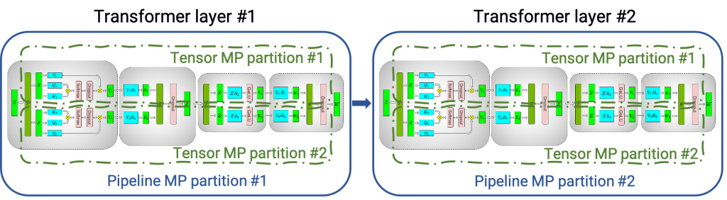

 This is the second part of a two-part series about NVIDIA tools that allow you to run large transformer models for accelerated inference. For an introduction to…
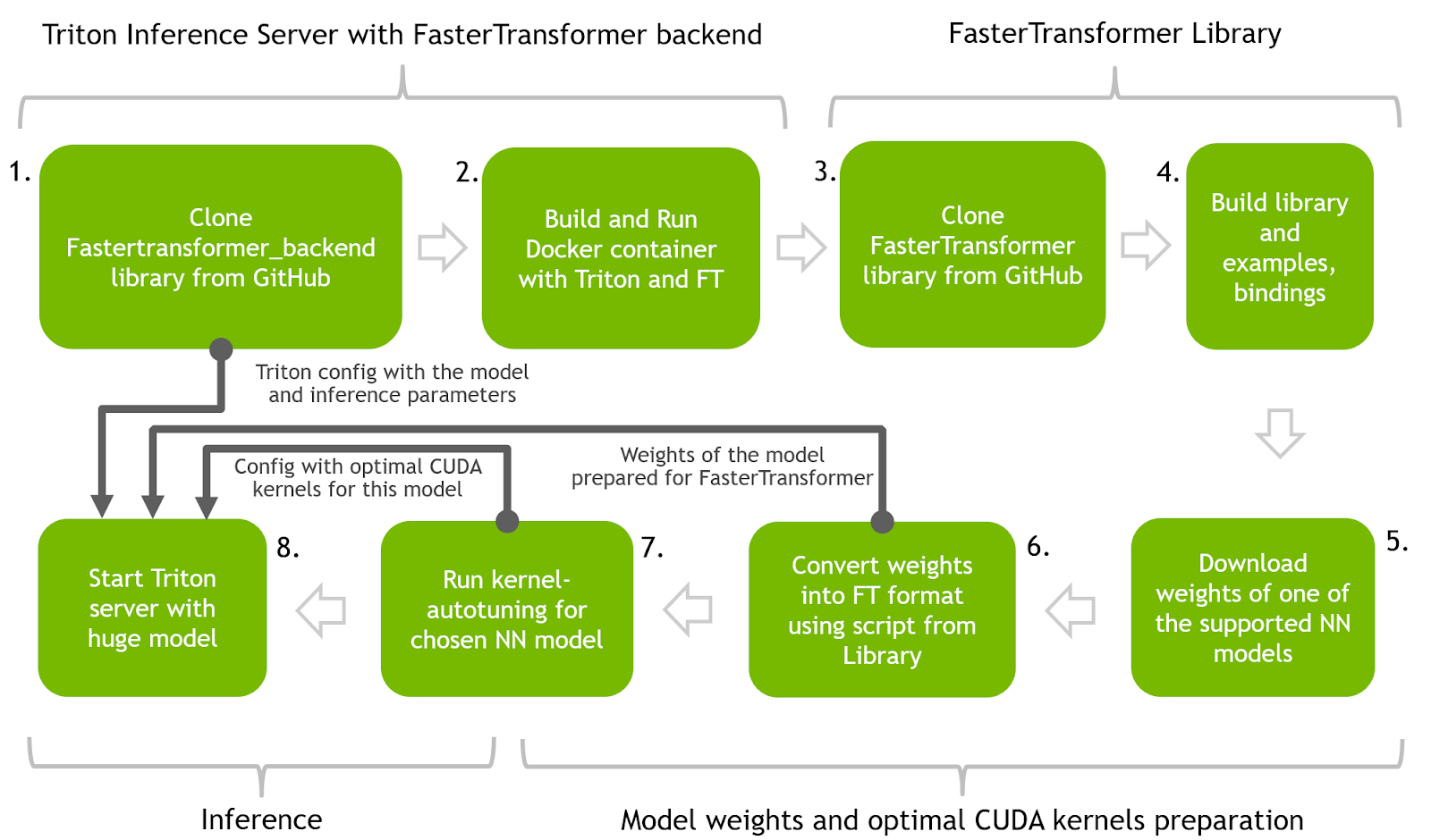


