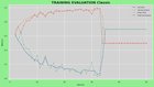
I was training a Image Classification Model with tensorflow. My training worked great until Epoch 34 where it suddenly dropped. Does anyone know what could be the reason for it?
How do I iterate through a custom dataset using image_dataset_from_directory? I’m trying to print the labels one by one, but it’s loading the images in batches. Is there any way the data can be loaded in without batches? My labels are one-hot encoded.
Researchers at NVIDIA have developed methods to improve and accelerate sampling from diffusion models, a novel and powerful class of generative models.
This is part of a series on how NVIDIA researchers have developed methods to improve and accelerate sampling from diffusion models, a novel and powerful class of generative models. Part 2covers three new techniques for overcoming the slow sampling challenge in diffusion models.
Generative models are a class of machine learning methods that learn a representation of the data they are trained on and model the data itself. They are typically based on deep neural networks. In contrast, discriminative models usually predict separate quantities given the data.
Generative models allow you to synthesize novel data that is different from the real data but still looks just as realistic. A designer could train a generative model on images of cars and then let the resulting generative AI computationally dream up novel cars with different looks, accelerating the artistic prototyping process.
Deep generative learning has become an important research area in the machine learning community and has many relevant applications. Generative models are widely used for image synthesis and various image-processing tasks, such as editing, inpainting, colorization, deblurring, and superresolution.
Generative models have the potential to streamline the workflow of photographers and digital artists and enable new levels of creativity. Similarly, they might allow content creators to efficiently generate virtual 3D content for games, animated movies, or the metaverse.
Deep learning-based speech and language synthesis have already found their way into consumer products. Fields such as medicine and healthcare may also benefit from generative models, such as methods that generate molecular drug candidates to fight disease.
The data representations learned by the neural networks of generative models, as well as the synthesized data, can often be used for training and fine-tuning other downstream machine learning models for different tasks, especially when labeled data is scarce.
Generative learning trilemma
For a wide adoption in real-world applications, generative models should ideally satisfy the following key requirements:
High-quality sampling: Many applications, especially those directly interacting with users, require high generation quality. For example, in speech generation, poor speech quality is difficult to understand. Similarly, in image modeling, the desired outputs are visually indistinguishable from natural images.
Mode coverage and sample diversity: If the training data contains a complex or large amount of diversity, a good generative model should successfully capture such diversity without sacrificing generation quality.
Fast and computationally inexpensive sampling: Many interactive applications require fast generation, such as real-time image editing.
While most current methods in deep generative learning focus on high-quality generation, the second and third requirements are highly important as well.
A faithful representation of the data’s diversity is crucial to avoid missing minority modes in the data distribution. This helps reduce undesired biases in the learned models.
On the other hand, in many applications, the long tails of the data distribution are particularly interesting. For instance, in traffic modeling, it is precisely the rare scenarios that are of interest, those that correspond to dangerous driving or accidents.
Reducing computational complexity and sampling time not only enables interactive, real-time applications. It also lessens the environmental footprint of running the expensive deep neural networks that underlie generative models by decreasing the overall power usage required for generation.
In this post, we identify the challenge imposed by these three requirements as the generative learning trilemmaas existing methods usually make trade-offs and cannot satisfy all requirements simultaneously.
Figure 1. Generative learning trilemma
Generative learning with diffusion models
Recently, diffusion models have emerged as a powerful class of generative learning methods. These models,, also known as denoising diffusion models or score-based generative models, demonstrate surprisingly high sample quality, often outperforming generative adversarial networks. They also feature strong mode coverage and sample diversity.
Diffusion models have already been applied to a variety of generation tasks, such as image, speech, 3D shape, and graph synthesis.
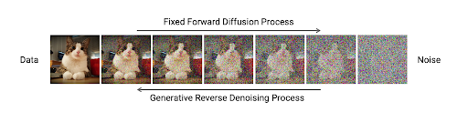
Diffusion models consist of two processes: forward diffusion and parametrized reverse.
A forward diffusion process maps data to noise by gradually perturbing the input data. This is formally achieved by a simple stochastic process that starts from a data sample and iteratively generates noisier samples using a simple Gaussian diffusion kernel. That is to say, at each step of this process, Gaussian noise is incrementally added to the data.
The second process is a parametrized reverse process that undoes the forward diffusion and performs iterative denoising. This process represents data synthesis and is trained to generate data by converting random noise into realistic data. It is also formally defined as a stochastic process, which iteratively denoises input images using trainable deep neural networks.
Both the forward and reverse processes often use thousands of steps for gradual noise injection and during generation for denoising.
Figure 2. Diffusion model processes moving to and from data and noise
Figure 2 shows that, in diffusion models, a fixed forward process gradually perturbs the data in a stepwise fashion towards fully random noise. A parametrized reverse process is learned to perform iterative denoising and to generate data, such as images, from noise.
Formally, denoting a data point such as an image by and its diffused version at timestep by , the forward process is defined by the following formula:
At each step, is sampled conditioned on using a Gaussian distribution with mean and variance . Here, is usually predefined and fixed, and is the total number of diffusion steps.
The reverse generative process is similarly defined in reverse order by:
In this formula, the denoising distribution is a Gaussian distribution whose mean is defined using a trainable neural network while its variance is often preset.
These processes are described in terms of discretized diffusion and denoising steps, indexed by a parameter , referred to as time along the forward and reverse processes. In particular, samples are generated iteratively one step at a time.
Continuous-time diffusion models
However, you can also study diffusion models in the limit of an infinite number of infinitely small time steps. This leads to continuous-time diffusion models where time flows continuously. In this case, the forward and reverse processes can be described using stochastic differential equations (SDEs).
A fixed forward SDE smoothly transforms a data sample into random noise. One option for such an SDE is as follows:
As before, denotes the data, and and represent the infinitesimal updates of data and time . Furthermore, is a noise process that corresponds to Gaussian noise injection, slowly perturbing the data. is now a continuous function of time . Furthermore, a corresponding generative SDE that is solved in the reverse direction along time maps noise to data:
Although discrete-time and continuous-time diffusion models may seem different, they share an almost identical generative process. In fact, it is easy to show that discrete-time diffusion models are special discretizations of continuous-time models.
Working with continuous-time diffusion models in practice is essentially a lot easier:
They are more generic and can be converted to discrete-time models using simple discretizations of time.
They are described using SDEs, which are well-studied in various scientific domains.
The generative SDEs can be solved using off-the-shelf numerical SDE solvers.
They can be converted to related ordinary differential equations (ODEs), which are also well-studied and easy to work with.
As mentioned earlier, diffusion models generate samples by following the reverse diffusion process that maps a simple base distribution, typically Gaussian, to the complex data distribution. This mapping, in continuous-time diffusion models represented by the generative SDE, is often complex due to the neural network approximating the score function.
Solving it with numerical integration techniques can require 1000s of calls to deep neural networks for sample generation. Because of this, diffusion models are often slow at sample generation, requiring minutes or even hours of computation time. This stands in stark contrast to competing techniques such as generative adversarial networks (GANs), which generate samples using only one call to a neural network.
Summary
Although diffusion models achieve high sample quality and diversity, they unfortunately fall short in sampling speed. This limits the wide adoption of diffusion models for practical real-world applications and has led to an active area of research on accelerated sampling from these models. In Part 2, we review three techniques developed at NVIDIA for overcoming the main limitation of diffusion models.
To learn more about the research that NVIDIA is advancing, see NVIDIA Research.
For more information about diffusion models, see the following resources:
Researchers at NVIDIA have developed methods to improve and accelerate sampling from diffusion models, a novel and powerful class of generative models.
This is part of a series on how researchers at NVIDIA have developed methods to improve and accelerate sampling from diffusion models, a novel and powerful class of generative models. Part 1introduced diffusion models as a powerful class for deep generative models and examined their trade-offs in addressing the generative learning trilemma.
While diffusion models satisfy both the first and second requirements of the generative learning trilemma, namely high sample quality and diversity, they lack the sampling speed of traditional GANs. In this post, we review three recent techniques developed at NVIDIA for overcoming the slow sampling challenge in diffusion models.
Latent space diffusion models
One of the main reasons why sampling from diffusion models is slow is that mapping from a simple Gaussian noise distribution to a challenging multimodal data distribution is complex. Recently, NVIDIA introduced the Latent Score-based Generative Model(LSGM), a new framework that trains diffusion models in a latent space rather than the data space directly.
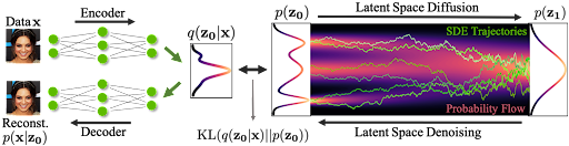
In LSGM, we leverage a variational autoencoder (VAE) framework to map the input data to a latent space and apply the diffusion model there. The diffusion model is then tasked with modeling the distribution over the latent embeddings of the data set, which is intrinsically simpler than the data distribution.
Novel data synthesis is achieved by first generating embeddings through drawing from a simple base distribution followed by iterative denoising, and then transforming this embedding using a decoder to data space (Figure 1).
Figure 1. Latent score-based generative model
Figure 1 shows that in the latent score-based generative model (LSGM),
Data is mapped to latent space through an encoder .
A diffusion process is applied in the latent space .
Synthesis starts from the base distribution .
It generates samples in latent space through denoising .
The samples are mapped from latent to data space using a decoder .
The model is trained end-to-end.
LSGM has several key advantages: synthesis speed, expressivity, and tailored encoders and decoders.
Synthesis speed
By pretraining the VAE with a Gaussian prior first, you can bring the latent encodings of the data distribution close to the Gaussian prior distribution, which is also the diffusion model’s base distribution. The diffusion model only has to model the remaining mismatch, resulting in a much less complex model from which sampling becomes easier and faster.
The latent space can be tailored accordingly. For example, we can use hierarchical latent variables and apply the diffusion model only over a subset of them or at a small resolution, further improving synthesis speed.
Expressivity
Training a regular diffusion model can be considered as training a neural ODE directly on the data. However, previous works found that augmenting neural ODEs, as well as other types of generative models, with latent variables often improves their expressivity.
We expect similar expressivity gains from combining diffusion models with a latent variable framework.
Tailored encoders and decoders
As you use the diffusion model in latent space, you can use carefully designed encoders and decoders mapping between latent and data space, further improving synthesis quality. The LSGM method can therefore be naturally applied to noncontinuous data.
Results
In principle, LSGM can easily model data such as text, graphs, and similar discrete or categorical data types by using encoder and decoder networks that transform this data into continuous latent representations and back.
Regular diffusion models that operate on the data directly could not easily model such data types. The standard diffusion framework is only well defined for continuous data, which can be gradually perturbed and generated in a meaningful manner.
Experimentally, LSGM achieves state-of-the-art Fréchet inception distance (FID), a standard metric to quantify visual image quality, on CIFAR-10 and CelebA-HQ-256, two widely used image generation benchmark data sets. On those data sets, it outperforms prior generative models, including GANs.
On CelebA-HQ-256, LSGM achieves a synthesis speed that is faster than previous diffusion models by two orders of magnitude. LSGM requires only 23 neural network calls when modeling the CelebA-HQ-256 data, compared to previous diffusion models trained on the data space that often rely on hundreds or thousands of network calls.
Video 1. Sequence generated by randomly traversing the latent space of LSGM.
Critically damped Langevin diffusion
A crucial ingredient in diffusion models is the fixed forward diffusion process to gradually perturb the data. Together with the data itself, it uniquely determines the difficulty of learning the denoising model. Hence, can we design a forward diffusion that is particularly easy to denoise and therefore leads to faster and higher-quality synthesis?
Diffusion processes like the ones employed in diffusion models are well studied in areas such as statistics and physics, where they are important in various sampling applications. Taking inspiration from these fields, we recently proposed critically damped Langevin diffusion (CLD)
In CLD, the data that must be perturbed are coupled to auxiliary variables that can be considered velocities, similar to velocities in physics in that they essentially describe how fast the data moves towards the diffusion model’s base distribution.
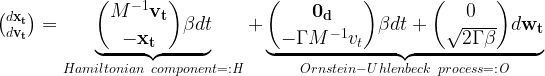
Like a ball that is dropped on top of a hill and quickly rolls into a valley on a relatively direct path accumulating a certain velocity, this physics-inspired technique helps the data to diffuse quickly and smoothly. The forward diffusion SDE that describes CLD is as follows:
Here, denotes the data and the velocities. , , and are parameters that determine the diffusion as well as the coupling between velocities and data. Furthermore, is a Gaussian white noise process, responsible for noise injection, as seen in the formula.
CLD can be interpreted as a combination of two different terms. First is an Ornstein-Uhlenback process, the particular kind of noise injection process used here, which acts on the velocity variables .
Second, the data and velocities are coupled to each other as in Hamiltonian dynamics, such that the noise injected into the velocities also affects the data . Hamiltonian dynamics provides a fundamental description of the mechanics of physical systems, like the ball rolling down a hill from the example mentioned earlier.
Figure 2 shows how data and velocity diffuse in CLD for a simple one-dimensional toy problem:
Figure 2. In critically-damped Langevin diffusion, the data xt is augmented with a velocity vt. A diffusion coupling xt and vt is run in the joint data-velocity space (probabilities in red). Noise is injected only into vt. This leads to smooth diffusion trajectories (green) for the data xt.
At the beginning of the diffusion, we draw a random velocity from a simple Gaussian distribution and the full diffusion then takes place in the joint data-velocity space. When looking at the evolution of the data (lower right in the figure), the model diffuses in a significantly smoother manner than for previous diffusions.
Intuitively, this should also make it easier to denoise and invert the process for generation. We obtain this behavior only for a particular choice of the diffusion parameters and , specifically for . This configuration is known as critical damping in physics and corresponds to a special case of a broader class of stochastic dynamical systems known as Langevin dynamics—hence the name critically damped Langevin diffusion.
We can also visualize how images evolve in the high-dimensional joint data-velocity space, both during forward diffusion and generation:
Figure 3. CLD’s forward diffusion and the reverse-time synthesis processes
At the top of Figure 3, we visualize how a one-dimensional data distribution together with the velocity diffuses in the joint data-velocity space and how generation proceeds in the reverse direction. We sample three different diffusion trajectories and also show the projections into data and velocity space on the right. At the bottom, we visualize a corresponding diffusion and synthesis process for image generation. We see that the velocities “encode” the data at intermediate times .
Using CLD when training generative diffusion models leads to two key advantages:
Simpler score function and training objective
Accelerated sampling with tailored SDE solvers
Simpler score function and training objective
In regular diffusion models, the neural network is tasked with learning the score function of the diffused data distribution. In CLD-based models, in contrast, we are tasked with learning , the conditional score function of the velocity given the data. This is a consequence of injecting noise only into the velocity variables.
However, as the velocity always follows a smoother distribution than the data itself, this is an easier learning problem. The neural networks used in CLD-based diffusion models can be simpler, while still achieving high generative performance. Related to that, we can also formulate an improved and more stable training objective tailored to CLD-based diffusion models.
Accelerated sampling with tailored SDE solvers
To integrate CLD’s reverse-time synthesis SDE, you can derive tailored SDE solvers for more efficient denoising of the smoother forward diffusion arising in CLD. This results in accelerated synthesis.
Experimentally, for the widely used CIFAR-10 image modeling benchmark, CLD outperforms previous diffusion models in synthesis quality for similar neural network architectures and sampling compute budgets. Furthermore, CLD’s tailored SDE solver for the generative SDE significantly outperforms solvers such as Euler–Maruyama, a popular method to solve the SDEs arising in diffusion models, in generation speed. For more information, see Score-Based Generative Modeling with Critically-Damped Langevin Diffusion.
Figure 4. Synthesized CIFAR-10 images generated by a diffusion model based on critically damped Langevin diffusion.
We’ve shown that you can improve diffusion models by merely designing their fixed forward diffusion process in a careful manner.
Denoising diffusion GANs
So far, we’ve discussed how to accelerate sampling from diffusion models by moving the training data to a smooth latent space as in LSGM or by augmenting the data with auxiliary velocity variables and designing an improved forward diffusion process as in CLD-based diffusion models.
However, one of the most intuitive ways to accelerate sampling from diffusion models is to directly reduce the number of denoising steps in the reverse process. In this part, we go back to discrete-time diffusion models, trained in the data space and analyze how the denoising process behaves as you reduce the number of denoising steps and perform large steps.
In a recent study, we observed that diffusion models commonly assume that the learned denoising distributions in the reverse synthesis process can be approximated by Gaussian distributions. However, it is known that the Gaussian assumption holds only in the infinitesimal limit of many small denoising steps, which ultimately leads to the slow synthesis of diffusion models.
When the reverse generative process uses larger step sizes (has fewer denoising steps), we need a non-Gaussian, multimodal distribution for modeling the denoising distribution .
Intuitively, in image synthesis, the multimodal distribution arises from the fact that multiple plausible and clean images may correspond to the same noisy image. Because of this multimodality, simply reducing the number of denoising steps, while keeping the Gaussian assumption in the denoising distributions, hurts generation quality.
Figure 5.(top) Evolution of a 1D data distribution q(x0) according to the forward diffusion process. (bottom) Visualizations of the true denoising distribution when conditioning on a fixed x5 with varying step sizes shown in different colors.
In Figure 5, the true denoising distribution for a small step size (shown in yellow) is close to a Gaussian distribution. However, it becomes more complex and multimodal as the step size increases.
Inspired by the preceding observation, we propose to parametrize the denoising distribution with an expressive multimodal distribution to enable denoising with large steps. In particular, we introduce a novel generative model, Denoising Diffusion GAN, in which the denoising distributions are modeled with conditional GANs (Figure 6).
Figure 6. Denoising diffusion process
Generative denoising diffusion models typically assume that the denoising distribution can be modeled by a Gaussian distribution. This assumption holds only for small denoising steps, which in practice translates to thousands of denoising steps in the synthesis process.
In our Denoising Diffusion GANs, we represent the denoising model using multimodal and complex conditional GANs, enabling us to efficiently generate data in as few as two steps.
Denoising Diffusion GANs are trained using an adversarial training setup (Figure 7). Given a training image , we use the forward Gaussian diffusion process to sample from both and , the diffused samples at two successive steps.
Given , our conditional denoising GAN first stochastically generates and then uses the tractable posterior distribution to generate by adding back noise. A discriminator is trained to distinguish between the real and the generated pairs and provides feedback to learn the conditional denoising GAN.
After training, we generate novel instances by sampling from noise and iteratively denoising it in few steps using our Denoising Diffusion GAN generator.
Figure 7. Training process of Denoising Diffusion GAN
We train a conditional GAN generator to denoise inputs using an adversarial loss for different steps in the diffusion process.
Advantages over traditional GANs
Why not just train a GAN that can generate samples in one shot using a traditional setup, in contrast to our model that iteratively generates samples by denoising? Our model has several advantages over traditional GANs.
GANs are known to suffer from training instabilities and mode collapse. Some possible reasons include the difficulty of directly generating samples from a complex distribution in one shot, as well as overfitting problems when the discriminator only looks at clean samples.
In contrast, our model breaks the generation process into several conditional denoising diffusion steps in which each step is relatively simple to model, due to the strong conditioning on . The diffusion process smoothens the data distribution, making the discriminator less likely to overfit.
We observe that our model exhibits better training stability and mode coverage. In image generation, we observe that our model achieves sample quality and mode coverage competitive with diffusion models while requiring only as few as two denoising steps.It achieves up to 2,000x speed-up in sampling compared to regular diffusion models. We also find that our model significantly outperforms state-of-the-art traditional GANs in sample diversity, while being competitive in sample fidelity.
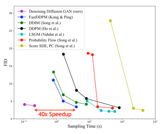
Figure 8. Sample quality vs. sampling time for different diffusion-based generative models
Figure 8 shows sample quality (as measured by Fréchet inception distance; lower is better) compared to sampling time for different diffusion-based generative models for the CIFAR-10 image modeling benchmark. Denoising Diffusion GANs achieve a speedup of several orders of magnitude compared to other diffusion models while maintaining similar synthesis quality.
Conclusion
Diffusion models are a promising class of deep generative models due to their combination of high-quality synthesis and strong diversity and mode coverage. This is in contrast to methods such as regular GANs, which are popular but often suffer from limited sample diversity. The main drawback of diffusion models is their slow synthesis speed.
In this post, we presented three recent techniques developed at NVIDIA that successfully address this challenge. Interestingly, they each approach the problem from different perspectives, analyzing the different components of diffusion models:
Latent space diffusion models essentially simplify the data itself, by first embedding it into a smooth latent space, where a more efficient diffusion model can be trained.
Critically damped Langevin diffusion is an improved forward diffusion process that is particularly well suited for easier and faster denoising and generation.
Denoising diffusion GANs directly learn a significantly accelerated reverse denoising process through expressive multimodal denoising distributions.
We believe that diffusion models are uniquely well-suited for overcoming the generative learning trilemma, in particular when using techniques like the ones highlighted in this post. These techniques can also be combined, in principle.
In fact, diffusion models have already led to significant progress in deep generative learning. We anticipate that they will likely find practical use in areas such as image and video processing, 3D content generation and digital artistry, and speech and language modeling. They will also find use in fields such as drug discovery and material design, as well as various other important applications. We think that diffusion-based approaches have the potential to power the next generation of leading generative models.
I trained a model on MNIST, but I get an error when trying to use model.predict on a single image. Apparently keras model.predict can only take in batches of images. Why? Is there any way around this?
This week In the NVIDIA Studio, we’re launching the April NVIDIA Studio Driver with optimizations for the most popular 3D apps, including Unreal Engine 5, Cinema4D and Chaos Vantage. The driver also supports new NVIDIA Omniverse Connectors from Blender and Redshift.
Take a deep dive into the integrated cloud-ready infrastructure solution from Red Hat and NVIDIA
The IT world is moving to cloud, and cloud is built on containers managed with Kubernetes. We believe the next logical step is to accelerate this infrastructure with data processing units (DPUs) for greater performance, efficiency, and security.
Red Hat and NVIDIA are building an integrated cloud-ready infrastructure solution with the management and automation of Red Hat OpenShift combined with the acceleration, workload isolation, and security capabilities of NVIDIA BlueField DPUs.
Benefits of Red Hat OpenShift
Many popular cloud infrastructure projects use containers managed by Kubernetes. However, implementing Kubernetes can be a heavy lift, especially for organizations that cannot devote dedicated staff to becoming Kubernetes experts.
Red Hat OpenShift provides a powerful set of capabilities for managing Kubernetes containers as well as application deployment, updates, and lifecycle management. OpenShift includes automation and security tools, as well as a supported open-source model to make cloud infrastructure more affordable, reliable, and scalable.
According to a 2021 Red Hat survey, Kubernetes is used for over 85% of container orchestration projects, and Red Hat OpenShift is the most popular choice for hybrid and multicloud Kubernetes deployments. OpenShift is the industry’s leading enterprise Kubernetes platform, used by more than 50% of commercial banks, telecommunications companies, and airlines on the Fortune 500.
It is clear that most enterprises want a supported Kubernetes model, and Red Hat OpenShift is one of the most popular choices.
How a DPU works
A DPU offloads, accelerates, and isolates infrastructure workloads from the server’s CPU. For example, the BlueField DPU can offload networking, network virtualization, data encryption, and time synchronization tasks from the CPU and run them on purpose-built silicon.
Other infrastructure software, such as remote management, firewall agents, network control plane, and storage virtualization, can run on BlueField’s Arm processor cores. Doing so frees up the server’s CPU cores that can instead run applications and tenant workloads.
This functionality also isolates infrastructure and security workloads in a separate domain. The result is a set of servers that run more applications with faster networking, increasing the efficiency and security of the data center.
In a typical cloud infrastructure, the network traffic traverses both physical servers and containers running on these servers. This requires a packet switching solution within each server, and to gain maximum efficiency, the application containers need a way to talk to the accelerated networking offloads of the DPU.
The traditional way is to go through Kubernetes and Open Virtual Network (OVN) to access the Open Virtual Switch (Open vSwitch or OVS). OVN provides network abstraction and the default deployment strategy is to run both OVN and OVS on the host server’s CPU.
However, this method consumes a significant number of CPU cores as the network speeds increase beyond 10 Gbps. A solution is needed for Kubernetes to run the OVN and OVS functionality on the DPU so that all the packet switching, header rewrites, encapsulation/decapsulation, and packet filtering can be done on networking hardware instead of in software on the CPU.
Increasing networking integration between Red Hat and NVIDIA
Red Hat and NVIDIA have collaborated to integrate the management power of OpenShift with the acceleration capabilities of the DPU.
The first stage of integration started in 2018 with Red Hat Enterprise Linux offloading network traffic to the NVIDIA ConnectX SmartNIC. The networking data plane–using OVS or DPDK–was running on the SmartNIC ASIC but the networking control plane was still running entirely in software on the X86 CPU.
Figure 1. OpenStack SDN controller, running on Red Hat Enterprise Linux, offloads the networking data plane to the NVIDIA ConnectX SmartNIC through OVS while the control plane runs on the X86 CPU.
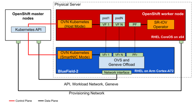
In this solution, the networking data plane with overlay offload (OVS and Geneve Offload) and the networking control plane (in the OVN Kubernetes pod) were running on the DPU with Red Hat Enterprise Linux. The major OpenShift components, including Red Hat Enterprise Linux CoreOS remained on the x86 CPU.
Figure 2. Red Hat OpenShift, running on Red Hat Enterprise Linux CoreOS, offloads both the networking data plane and control plane to the BlueField-2 DPU, via OVN and OVS. The DPU is running Red Hat Enterprise Linux on its Arm cores.
In the deployment scenario in Figure 2, the BlueField-2 does the heavy lifting in the following areas:
The host CPU and container see only simple unencapsulated, unencrypted packets and the CPU does not need to perform any of these tasks because they are offloaded to the DPU. This level of offload reduced CPU utilization by 70%, freeing up substantial CPU power on each server to run additional business/tenant workloads.
Running OpenShift on the DPU
As presented at GTC 2022, Red Hat and NVIDIA have taken the next step, moving OpenShift, including Red Hat Enterprise Linux CoreOS, to run on the Arm cores of the BlueField DPU for the Red Hat OpenShift two cluster design that includes separate tenant and infrastructure clusters.
Red Hat Enterprise Linux CoreOS is the supported operating system for the OpenShift control plane, or master and worker nodes. This is the portion of OpenShift that performs scheduling, maintenance, upgrades, and cluster automation. It includes container management tools and security hardening to make it more resistant to hackers, and it now runs on both the host x86 CPU and on the DPU Arm cores.
BlueField DPUs running OpenShift OVS and OVN containers and Red Hat Enterprise Linux CoreOS on the various host servers form an infrastructure worker cluster. Meanwhile, OpenShift running on the x86 CPUs manages the tenant pods and clusters.
Offloading the OpenShift infrastructure cluster software to run on the BlueField Arm cores instead of on the host x86 cores provides additional x86 CPU savings, higher performance, and stronger security isolation.
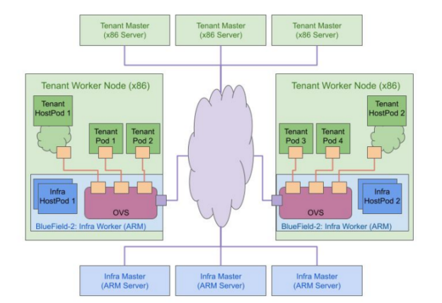
Figure 3. Starting with Red Hat OpenShift 4.10, you can run OpenShift on both the x86 CPUs to manage the tenants and on the BlueField DPU Arm cores to manage the cluster infrastructure.
The cloud-native, software-defined networking is a good example of a BlueField DPU use case where OVN and OVS are running on and offloaded by the BlueField DPU in an OpenShift environment. Many other infrastructure services, such as network encryption, firewall agents, virtual routers, telemetry agents, and so on, can also be run on the DPU for an even greater benefit.
Significant cost savings benefits from OpenShift Offload on DPU
To understand the impact of the DPU offloads on reducing the data center costs, NVIDIA and Red Hat put together a TCO model for a mid-sized data center with 51K servers. We considered this data center to be supporting 1M applications, each application needing 10K packets per second (PPS) of switching performance.
The server with no DPU running the virtual switching entirely in software achieved only 350k PPS.
The server with a DPU that offloads OVN and OVS to the DPU achieved 54x times higher performance of 18.7 million PPS per server.
Offloading virtual switching to the DPU also saved eight CPU cores per server. Based on this testing, the TCO model yielded amazing savings of $68.5M of CapEx. These savings are recognized by requiring 10K fewer DPU-enhanced servers due to much higher networking performance and CPU core savings per server.
We see power savings due to the smaller server footprint, which ultimately results in a better TCO model with the DPU-based servers. These TCO savings will get even better as we offload additional functions such as load balancers, firewalls, encryption, web servers, and so on to the DPUs, ultimately achieving amazing efficiency for cloud-ready data centers.
Solution roadmap and deploying OpenShift on BlueField
The two-cluster OpenShift architecture running OpenShift on BlueField is now available as a developer preview or early trial in OpenShift 4.10, and is expected to become generally available in 2022.
But the NVIDIA and Red Hat teams aren’t stopping here. We are planning to test the offloading of network traffic encryption/decryption as that is a CPU-intensive task.
BlueField-2 DPU can offload IPsec encryption/decryption at up to 100 Gbps and TLS encryption/decryption at up to 200 Gbps.
BlueField-3 is expected to support IPSec, TLS and MACsec at even higher speeds.
Implementation of line-rate encryption offload from OpenShift to the DPU will improve data security for tenants and help you move closer to a zero-trust security stance.
Other potential integrations with the DPU include more sophisticated software-defined networking offloads, running a firewall agent on BlueField, precision time synchronization, video streaming with packet pacing, and using the DPU to collect telemetry data.
BlueField-2 DPUs are available now from NVIDIA and the BlueField-3 DPU will start sampling later in 2022. In addition, BlueField DPUs will soon be available for testing in the NVIDIA LaunchPad cloud service.
If you would like to test or develop on Red Hat OpenShift running with the NVIDIA BlueField DPU, please indicate your interest.
Summary
If your organization seeks to embrace cloud-native computing in data centers, the combination of NVIDIA BlueField DPUs, Red Hat Enterprise Linux, and Red Hat OpenShift provides an efficient and innovative open, hybrid-cloud platform with new security features. This powerful platform delivers hardware acceleration capabilities to run critical software-defined networking, storage, and security functions.
Now more server resources can be allocated to run cloud-native workloads, as well as traditional business applications.
For more information, see the following resources:
I’m a newbee in the machine learning frameworks. When I’m learning machine learning frameworks such as TensorFlow, PyTorch, and MindSpore, I’m confused between accuracy and precision. What is the difference when we say to improve model accuracy and to improve model precision? Can you help me to figure it out? Thanks


 Join NVIDIA Jetson experts on Tuesday, May 10 for a webinar and Q&A about JetPack 5.0, the latest release supporting the Jetson platform.
 Researchers at NVIDIA have developed methods to improve and accelerate sampling from diffusion models, a novel and powerful class of generative models.
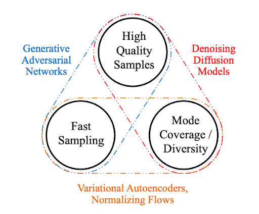
 and its diffused version at timestep
  by
by  , the forward process is defined by the following formula:
 using a Gaussian distribution with mean
  and variance
  . Here,
  is the total number of diffusion steps.
 is a Gaussian distribution whose mean is defined using a trainable neural network
  while its variance is often preset.
 and
and  represent the infinitesimal updates of data and time
  is a noise process that corresponds to Gaussian noise injection, slowly perturbing the data.
  is now a continuous function of time
 is mapped to latent space through an encoder
  .
. .
. .
.  in latent space through denoising
  .
.  .
. 
 the velocities.
  ,
,  , and
, and  are parameters that determine the diffusion as well as the coupling between velocities and data. Furthermore,
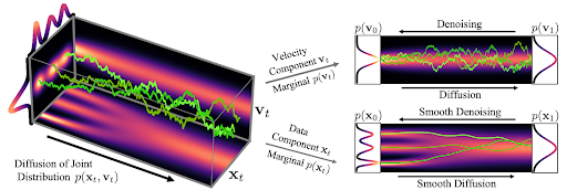
 . This configuration is known as critical damping in physics and corresponds to a special case of a broader class of stochastic dynamical systems known as Langevin dynamics—hence the name critically damped Langevin diffusion.
 of the diffused data distribution. In CLD-based models, in contrast, we are tasked with learning
  , the conditional score function of the velocity given the data. This is a consequence of injecting noise only into the velocity variables.
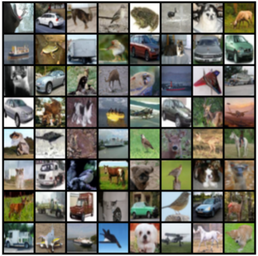
 in the reverse synthesis process can be approximated by Gaussian distributions. However, it is known that the Gaussian assumption holds only in the infinitesimal limit of many small denoising steps, which ultimately leads to the slow synthesis of diffusion models.
 and then uses the tractable posterior distribution
  to generate
  by adding back noise. A discriminator is trained to distinguish between the real
  and the generated
  pairs and provides feedback to learn the conditional denoising GAN.
") Take a deep dive into the integrated cloud-ready infrastructure solution from Red Hat and NVIDIA
Take a deep dive into the integrated cloud-ready infrastructure solution from Red Hat and NVIDIA 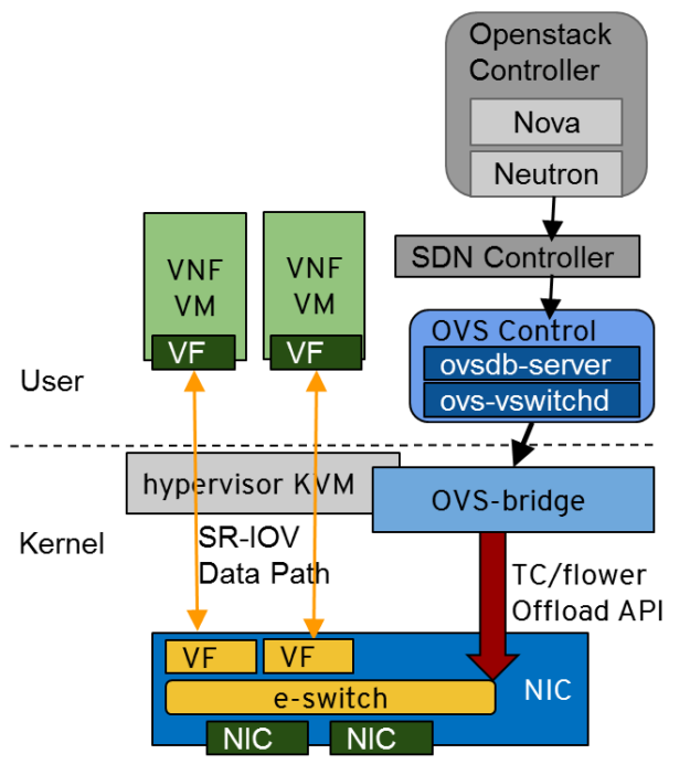

