Posted by Brian Lester, AI Resident and Noah Constant, Senior Staff Software Engineer, Google Research
Large pre-trained language models, which are continuing to grow in size, achieve state-of-art results on many natural language processing (NLP) benchmarks. Since the development of GPT and BERT, standard practice has been to fine-tune models on downstream tasks, which involves adjusting every weight in the network (i.e., model tuning). However, as models become larger, storing and serving a tuned copy of the model for each downstream task becomes impractical.
An appealing alternative is to share across all downstream tasks a single frozen pre-trained language model, in which all weights are fixed. In an exciting development, GPT-3 showed convincingly that a frozen model can be conditioned to perform different tasks through “in-context” learning. With this approach, a user primes the model for a given task through prompt design, i.e., hand-crafting a text prompt with a description or examples of the task at hand. For instance, to condition a model for sentiment analysis, one could attach the prompt, “Is the following movie review positive or negative?” before the input sequence, “This movie was amazing!”
Sharing the same frozen model across tasks greatly simplifies serving and allows for efficient mixed-task inference, but unfortunately, this is at the expense of task performance. Text prompts require manual effort to design, and even well-designed prompts still far underperform compared to model tuning. For instance, the performance of a frozen GPT-3 175B parameter model on the SuperGLUE benchmark is 5 points below a fine-tuned T5 model that uses 800 times fewer parameters.
In “The Power of Scale for Parameter-Efficient Prompt Tuning”, presented at EMNLP 2021, we explore prompt tuning, a more efficient and effective method for conditioning frozen models using tunable soft prompts. Just like engineered text prompts, soft prompts are concatenated to the input text. But rather than selecting from existing vocabulary items, the “tokens” of the soft prompt are learnable vectors. This means a soft prompt can be optimized end-to-end over a training dataset. In addition to removing the need for manual design, this allows the prompt to condense information from datasets containing thousands or millions of examples. By comparison, discrete text prompts are typically limited to under 50 examples due to constraints on model input length. We are also excited to release the code and checkpoints to fully reproduce our experiments.
Prompt tuning retains the strong task performance of model tuning, while keeping the pre-trained model frozen, enabling efficient multitask serving.
Prompt Tuning To create a soft prompt for a given task, we first initialize the prompt as a fixed-length sequence of vectors (e.g., 20 tokens long). We attach these vectors to the beginning of each embedded input and feed the combined sequence into the model. The model’s prediction is compared to the target to calculate a loss, and the error is back-propagated to calculate gradients, however we only apply these gradient updates to our new learnable vectors — keeping the core model frozen. While soft prompts learned in this way are not immediately interpretable, at an intuitive level, the soft prompt is extracting evidence about how to perform a task from the labeled dataset, performing the same role as a manually written text prompt, but without the need to be constrained to discrete language.
Our codebase, implemented in the new JAX-based T5X framework, makes it easy for anyone to replicate this procedure, and provides practical hyperparameter settings, including a large learning rate (0.3), which we found was important for achieving good results.
Since soft prompts have a small parameter footprint (we train prompts with as few as 512 parameters), one can easily pass the model a different prompt along with each input example. This enables mixed-task inference batches, which can streamline serving by sharing one core model across many tasks.
Left: With model tuning, incoming data are routed to task-specific models. Right: With prompt tuning, examples and prompts from different tasks can flow through a single frozen model in large batches, better utilizing serving resources.
Improvement with Scale When evaluated on SuperGLUE and using a frozen T5 model, prompt tuning significantly outperforms prompt design using either GPT-3 or T5. Furthermore, as model size increases, prompt tuning catches up to the performance level of model tuning. Intuitively, the larger the pre-trained model, the less of a “push” it needs to perform a specific task, and the more capable it is of being adapted in a parameter-efficient way.
As scale increases, prompt tuning matches model tuning, despite tuning 25,000 times fewer parameters.
The effectiveness of prompt tuning at large model scales is especially important, since serving separate copies of a large model can incur significant computational overhead. In our paper, we demonstrate that larger models can be conditioned successfully even with soft prompts as short as 5 tokens. For T5 XXL, this means tuning just 20 thousand parameters to guide the behavior of an 11 billion parameter model.
Resilience to Domain Shift Another advantage of prompt tuning is its resilience to domain shift. Since model tuning touches every weight in the network, it has the capacity to easily overfit on the provided fine-tuning data and may not generalize well to variations in the task at inference time. By comparison, our learned soft prompts have a small number of parameters, so the solutions they represent may be more generalizable.
To test generalizability, we train prompt tuning and model tuning solutions on one task, and evaluate zero-shot on a closely related task. For example, when we train on the Quora Question Pairs task (i.e., detecting if two questions are duplicates) and evaluate on MRPC (i.e., detecting if two sentences from news articles are paraphrases), prompt tuning achieves +3.2 points higher accuracy than model tuning.
Train
Eval
Tuning
Accuracy
F1
QQP
MRPC
Model
73.1 ±0.9
81.2 ±2.1
Prompt
76.3 ±0.1
84.3 ±0.3
MRPC
QQP
Model
74.9 ±1.3
70.9 ±1.2
Prompt
75.4 ±0.8
69.7 ±0.3
On zero-shot domain transfer between two paraphrase detection tasks, prompt tuning matches or outperforms model tuning, depending on the direction of transfer.
Looking Forward Prompt-based learning is an exciting new area that is quickly evolving. While several similar methods have been proposed — such as Prefix Tuning, WARP, and P-Tuning — we discuss their pros and cons and demonstrate that prompt tuning is the simplest and the most parameter efficient method.
In addition to the Prompt Tuning codebase, we’ve also released our LM-adapted T5 checkpoints, which we found to be better-suited for prompt tuning compared to the original T5. This codebase was used for the prompt tuning experiments in FLAN, and the checkpoints were used as a starting point for training the BigScience T0 model. We hope that the research community continues to leverage and extend prompt tuning in future research.
Acknowledgements This project was a collaboration between Brian Lester, Rami Al-Rfou and Noah Constant. We are grateful to the following people for feedback, discussion and assistance: Waleed Ammar, Lucas Dixon, Slav Petrov, Colin Raffel, Adam Roberts, Sebastian Ruder, Noam Shazeer, Tu Vu and Linting Xue.
Sharpen your conversational AI, vehicle routing, or CUDA Python skills; learn how Metropolis boosts go-to-market efforts; find solutions for AI inference deployment.
Our weekly roundup covers the most recent software updates, learning resources, events, and notable news.
Learn to Deploy a Text Classification Model Using Riva (DLI)
This free, 30 minute, online course is self paced and includes a sample notebook from the NGC TAO Toolkit—Conversational AI collection, complete with a live GPU environment.
In this free one-hour course, participants will work through a demonstration of a common vehicle routing optimization problem at their own pace. Upon completion, participants will be able to preprocess input data for use by NVIDIA ReOpt routing solver, and compose variants of the problem that reflect real-world business constraints.
Fundamentals of Accelerated Computing with CUDA Python (DLI)
This Deep Learning Institute workshop teaches you the fundamental tools and techniques for running GPU-accelerated Python applications using CUDA GPUs and the Numba compiler. This workshop is being offered Feb, 23 from 9 am to 5 pm PT.
At the conclusion of the workshop, you’ll have an understanding of the fundamental tools and techniques for GPU-accelerated Python applications with CUDA and Numba, including:
GPU-accelerate NumPy ufuncs with a few lines of code.
Configure code parallelization using the CUDA thread hierarchy.
Write custom CUDA device kernels for maximum performance and flexibility.
Use memory coalescing and on-device shared memory to increase CUDA kernel bandwidth.
Learn How Metropolis Boosts Go-to-Market Efforts at a Developer Meetup
Join NVIDIA experts at developer meetups Feb. 16 and 17, and find out how the Metropolis program can grow your vision AI business and enhance go-to-market efforts.
Learn how:
Metropolis Validation Labs optimize your applications and accelerate deployments.
NVIDIA Fleet Command simplifies provisioning and management of edge deployments accelerating the time to scale from POC to production.
NVIDIA Launchpad provides easy access to GPU instances for faster POCs and customer trial
A Flexible Solution for Every AI Inference Deployment
Dive into NVIDIA inference solutions, including open-source NVIDIA Triton Inference Server and NVIDIA TensorRT, with a webinar and live Q&A, Feb. 23 at 10 a.m. PT.
Learn how:
To optimize, deploy, and scale AI models in production using Triton Inference Server and TensorRT.
Triton streamlines inference serving across multiple frameworks, across different query types (real-time, batch, streaming), on CPUs and GPUs, and with a model analyzer for efficient deployment.
To standardize workflows to optimize models using TensorRT and framework Integrations with PyTorch and TensorFlow.
Real-world customers are benefitting from Triton and TensorRT.
This post details CUDA’s new int128 support and how to implement decimal fixed-point arithmetic on top of it.
“Truth is much too complicated to allow anything but approximations.” — John von Neumann
The history of computing has demonstrated that there is no limit to what can be achieved with the relatively simple arithmetic implemented in computer hardware. But the “truth” that computers represent using finite-size numbers is fundamentally approximate. As David Goldberg wrote, “Squeezing infinitely many real numbers into a finite number of bits requires an approximate representation.” Floating point is the most widely used representation of real numbers, implemented in many processors, including GPUs. It is popular due to its ability to represent a large dynamic range of values and to trade off range and precision.
Unfortunately, floating point’s flexibility and range can cause trouble in applications where accuracy within a fixed range is more important: think dollars and cents. Binary floating point numbers cannot exactly represent every decimal value, and their approximation and rounding can lead to accumulation of errors that may be unacceptable in accounting calculations, for example. Moreover, adding very large and very small floating-point numbers can result in truncation errors. For these reasons, many currency and accounting computations are implemented using fixed-point decimal arithmetic, which stores a fixed number of fractional digits. Depending on the range required, fixed-point arithmetic may need a larger number of bits.
NVIDIA GPUs do not implement fixed-point arithmetic in hardware, but a GPU-accelerated software implementation can be efficient. In fact, RAPIDS cuDF library has provided efficient 32- and 64-bit fixed-point decimal numbers and computation for a while now. But some users of RAPIDS cuDF and GPU-accelerated Apache Spark need the higher range and precision provided by 128-bit decimals, and now NVIDIA CUDA 11.5 provides preview support of the 128-bit integer type(int128) that is needed to implement 128-bit decimal arithmetic.
In this post, after introducing CUDA’s new int128 support, we detail how we implemented decimal fixed-point arithmetic on top of it. We then demonstrate how 128-bit fixed-point support in RAPIDS cuDF enables key Apache Spark workloads to run entirely on GPU.
Introducing CUDA __int128
In NVIDIA CUDA 11.5, the NVCC offline compiler has added preview support for the signed and unsigned __int128 data types on platforms where the host compiler supports it. The nvrtc JIT compiler has also added support for 128-bit integers, but requires a command-line option, --device-int128, to enable this support. but requires a command-line option, –device-int128, to enable this support. Arithmetic, logical, and bitwise operations are all supported on 128-bit integers. Note that DWARF debug support for 128-bit integers is not available yet and will be available in a subsequent CUDA release. With the 11.6 release, cuda-gdb and Nsight Visual Studio Code Edition have added support for inspecting this new variable type.
NVIDIA GPUs compute integers in 32-bit quantities, so 128-bit integers are represented using four 32-bit unsigned integers. The addition, subtraction, and multiplication algorithms are straightforward and use the built-in PTX addc/madc instructions to handle multiple-precision values. Division and remainder are implemented using a simple O(n^2) division algorithm, similar to Algorithm 1.6 in Brent and Zimmermann’s book Modern Computer Arithmetic, with a few optimizations to improve the quotient selection step and minimize correction steps.One of the motivating use cases for 128-bit integers is using them to implement decimal fixed-point arithmetic. 128-bit decimal fixed-point support is included in the 21.12 release of RAPIDS libcudf. Keep reading to find out more about fixed-point arithmetic and how __int128 is used to enable high-precision computation.
Fixed-point Arithmetic
Fixed-point numbers represent real numbers by storing a fixed number of digits for the fractional part. Fixed-point numbers can also be used to “omit” the lower-order digits of integer values (i.e. if you want to represent multiples of 1000, you can use a base-10 fixed-point number with scale equal to 3). One easy way to remember the difference between fixed-point and floating point is that with fixed-point numbers, the decimal “point” is fixed, whereas in floating-point numbers the decimal “point” can float (move).
The basic idea behind fixed-point numbers is that even though the values being represented can have fractional digits (aka the 0.23 in 1.23), you actually store the value as an integer. To represent 1.23, for example, you can construct a fixed_point number with scale = -2 and value 123. This representation can be converted to a floating point number by multiplying the value by the radix raised to the scale. So in our example, 1.23 is produced by multiplying 123 (value) by 0.001 (10 (radix) to the power of -2 (scale)). When constructing a fixed-point number, the opposite occurs and you “shift” the value so that you can store it as an integer (with the floating point number 1.23 you would divide by 0.001 if you were using scale -2 (0.001 (10 (radix) to the power of -2 (scale))).
Note that fixed-point representations are not unique because you can choose multiple scales. For the example of 1.23, you can use any scale less than -2, such as -3 or -4. The only difference is that the number stored on disk will be different; 123 for scale -2, 1230 for scale -3 and 12300 for scale -4. When you know that your use case only requires a set number of decimal places, you should use the least precise (aka largest) scale possible to maximize the range of representable values. With scale -2 the range is roughly -20 to +20 million (with two decimal places), whereas with scale -3 the range is roughly -2 to +2 million (with three decimal places). If you know you are modeling money and you don’t need three decimal places, scale -2 is a much better option.
Another parameter of a fixed-point type is the base. In the examples in this post, and in RAPIDS cuDF, we use base 10, or decimal fixed point. Decimal fixed point is the easiest to think about because we are comfortable with decimal (base 10) numbers. The other common base for fixed-point numbers is base 2, also known as binary fixed point. This simply means that instead of shifting value by powers of 10, the scale shifts a value by powers of 2. You can see some examples of binary and decimal fixed-point values later in the “Examples” section.
Fixed point Vs floating point
Fixed Point
Floating Point
Narrower, static range
Wider, dynamic range
Exact representation avoids certain truncation and rounding errors
Truncation errors can occur
Keeps relative error constant
Approximate representation leads to certain truncation and rounding errors
Keeps relative error constant
Table 1: Comparison of floating point and fixed point.
Absolute error is the difference between the real value and its computer representation (in either fixed or floating point). Relative error is the ratio of the absolute error to the represented value.
To demonstrate issues with floating point representations that fixed point can address, let’s look at exactly how floating point is represented. A floating point number cannot represent all values exactly. For instance, the closest 32-bit floating point number to value 1.1 is 1.10000002384185791016 (see float.exposed to visualize this). The trailing “imprecision” can lead to errors when performing arithmetic operations. For example, 1.1 + 1.1 yields 2.20000004768371582031.
Figure 1: Visualization of 1.1 in floating-point.
In contrast, when using fixed-point representations, an integer is used to store the exact value. To represent 1.1 using a fixed-point number with a scale equal to -1, the value 11 is stored. Arithmetic operations are performed on the underlying integer, so adding 1.1 + 1.1 as fixed-point numbers simply adds 11 + 11 yielding 22, representing the value 2.2 exactly
Why is fixed-point arithmetic important?
As shown in the example preceding, fixed-point arithmetic avoids the precision and rounding errors inherent in floating point numbers while still providing the ability to represent fractional digits. Floating point provides a much larger range of values by keeping relative error constant. However, this means it can suffer from large absolute (truncation) errors when adding very large and very small numbers and run into rounding errors. Fixed-point representation always has the same absolute error at the cost of being able to represent a reduced range of values. If you know you need a specific precision after the decimal/binary point, then fixed point allows you to maintain accuracy of those digits without truncation even as the value grows, up to the limits of the range. If you need more range, you have to add more bits. Hence decimal128 becomes important for some users.
Lower Bound
Upper Bound
decimal32
-21474836.48
21474836.47
decimal64
-92233720368547758.08
92233720368547758.07
decimal128
-1701411834604692317 316873037158841057.28
1701411834604692317316 873037158841057.27
Table 2: Ranges for decimal32 with scale = -2.
There are many applications and use cases for fixed_point numbers. You can find a list of actual applications that use fixed_point numbers on Wikipedia
fixed_point in RAPIDS libcudf
Overview
The core of the RAPIDS libcudf `fixed_point` type is a simple class template.
template
class fixed_point {
  Rep _value;
  scale_type _scale;
}
The fixed_point class is templated on:
Rep: the representation of the fixed_point number (for example, the integer type used)
Rad: the Radix of the number (for example, base 2 or base 10)
The decimal32 and decimal64 types use int32_t and int64_t for the Rep, respectively and both have Radix::BASE_10. The scale is a strongly typed run-time variable (see Run-Time Scale and Strong Typing subsections below, etc).
The fixed_point type has several constructors (see Ways to Construct subsection below), explicit conversion operators to cast to both integral and floating point types, and a full complement of operators (addition, subtraction, etc.).
Sign of Scale
In most C++ fixed-point implementations (including RAPIDS libcudf’s), a negative scale indicates the number of fractional digits. A positive scale indicates the multiple that is representable (for example, if scale = 2 for a decimal32, multiples of 100 can be represented).
auto const number_with_pos_scale = decimal32{1.2345, scale_type{-2}}; // 1.23
auto const number_with_neg_scale = decimal32{12345,  scale_type{2}}; // 12300
Constructors
The following (simplified) constructors are provided in libcudf:
Where Rep is a signed integer type and T can be either an integral type or floating-point number.
Design and motivation
There are a number of design goals for libcudf’s fixed_point type. These include:
Need for a run-time scale
Consistency with potential standard C++ fixed_point types
Strong typing
These design motivations are detailed below.
Run-time scale and third-party fixed-point libraries
We studied eight existing fixed-point C++ libraries during the design phase. The primary reason for not using a third-party library is that all of the existing fixed-point types/libraries are designed with the scale being a compile-time parameter. This does not work for RAPIDS libcudf as it needs scale to be a run-time parameter.
While RAPIDS libcudf is a C++ library that can be used in C++ applications, it is also the backend for RAPIDs cuDF, which is a Python library. Python is an interpreted (rather than compiled, like C++) language. Moreover, cuDF must be able to read or receive fixed-point data from other data sources. This means that we do not know the scale of the fixed-point values at compile time. Therefore we need to have the fixed_point type in RAPIDS libcudf that has a run-time scale parameter.
The main library we referenced was CNL, the Compositional Numeric Library by John McFarlane that is currently the reference for an ISO C++ proposal to add fixed-point types to the C++ standard. We aim for the RAPIDS libcudf fixed_point type to be as similar as possible to the potentially standardized type. Here’s a simple comparison between RAPIDS libcudf and CNL.
using namespace numeric;
auto x = fixed_point{1.23, scale_type{-2}};
Or alternatively:
using namespace numeric;
auto x = decimal32{1.23, scale_type{-2}};
The most important difference to notice here is the -2 as a template (aka compile-time parameter) in the CNL example versus the scale_type{-2} as a run-time parameter in the RAPIDS libcudf example.
Strong typing
Strong typing has been incorporated into the design of the fixed_point type. Two examples of this are:
Using a scoped enumeration for Radix instead of an integer type
RAPIDS libcudf adheres to strong typing best practices and strongly typed APIs because of the protection and expressivity strong typing provides. I won’t go into the rabbit hole of weak compared to strong typing, but if you would like to read more about it there are many great resources, including Jonathon Bocarra’s Fluent C++ post on How typed C++ is, and why it matters.
Adding support for decimal128
RAPIDS libcudf 21.12 adds decimal128 as a supported fixed_point type. This required a number of changes, the first being the addition of the decimal128 type alias that relies on the __int128 type provided by CUDA 11.5.
using decimal32  = fixed_point;
using decimal64  = fixed_point;
using decimal128 = fixed_point;
This required a number of internal changes, including updating type traits functions, __int128_t specializations for certain functions, and adding support so that cudf::column_view and friends work with decimal128. The following simple examples demonstrate the use of libcudf APIs with decimal128 (note, all of these examples work the same for decimal32 and decimal64).
Examples
Simple currency
A simple currency example uses the decimal32 type provided by libcudf with scale -2 to represent exactly $17.29:
auto const money = decimal32{17.29, scale_type{-2}};
Summing large and small numbers
Fixed point is very useful when summing both large and small values. As a simple toy example, the following piece of code sums the powers of 10 from exponent -2 to 9.
template
auto sum_powers_of_10() {
    auto iota = std::views::iota(-2, 10);
    return std::transform_reduce(
        iota.begin(), iota.end(),
        T{}, std::plus{},
        [](auto e) -> T { return std::pow(10, e); });
}
Comparing 32-bit floating-point and decimal fixed point shows the following results:
Where decimal_type is a 32-bit base-10 fixed-point type. You can see an example of this using the CNL library on Godbolt here.
Avoiding floating-point rounding issues
An example of where floating-point values run into issues (in C++) is the following piece of code (see in Godbolt):
std::cout
The equivalent code in RAPIDS libcudf will not have the same issue (see on Github):
auto col = // decimal32 column with scale -5 and value 256.49999
auto result = cudf::round(input); // result is 256
The value of 256.4999 is not representable with a 32-bit binary float and therefore rounds to 256.5 before the std::roundf function is called. This problem can be avoided with fixed-point representation because 256.4999 is representable with any base-10 (decimal) type that has five or more fractional values of precision.
Binary versus decimal fixed point
// Decimal Fixed Point
using decimal32 = fixed_point;
auto const a = decimal32{17.29, scale_type{-2}}; // 17.29
auto const b = decimal32{4.2, scale_type{ 0}}; // 4
auto const c = decimal32{1729, scale_type{ 2}}; // 1700
// Binary Fixed Point
using binary32 = fixed_point;
auto const x = binary{17.29, scale_type{-2}}; // 17.25
auto const y = binary{4.2, scale_type{ 0}}; // 4
auto const z = binary{1729, scale_type{ 2}}; // 1728
decimal128
// Multiplying two decimal128 numbers
auto const x = decimal128{1.1, scale_type{-1});
auto const y = decimal128{2.2, scale_type{-1}};
auto const z = x * y; // 2.42 with scale equal to -2
// Adding two decimal128 numbers
auto const x = decimal128{1.1, scale_type{-1});
auto const y = decimal128{2.2, scale_type{-1}};
auto const z = x * y; // 3.3 with scale equal to -1
DecimalType in RAPIDS Spark
DecimalType in Apache Spark SQL is a data type that can represent Java BigDecimal values. SQL queries operating on financial data make significant use of the decimal type. Unlike the RAPIDS libcudf implementation of fixed-point decimal numbers, the maximum precision possible for DecimalType in Spark is limited to 38 bits. The scale, which is defined as the number of digits after the decimal point, is also capped at 38. This definition is the negative of the C++ scale. For example, a decimal value like 0.12345 has a scale of 5 in Spark but a scale of -5 in libcudf.
Spark closely follows the Apache Hive specification on precision calculations for operations and provides options to the user to configure precision loss for decimal operations. Spark SQL is aggressive about promoting precision of the result column when performing operations like aggregation, windowing, casting and so on This behavior in and of itself is what makes decimal128 extremely relevant to real-world queries and answers the question: “Why do we need support for high-precision decimal columns?”. Consider the example below, specifically the hash aggregate, which has a multiplication expression involving a decimal64 column, price, and a non-decimal column, quantity. Spark first casts the non-decimal column to an appropriate decimal column. It then determines the result precision, which is greater than the input precision. Therefore, it is quite common for the result precision to be a decimal128 value even if decimal64 inputs are involved.
scala> val queryDfGpu = readPar.agg(sum('price*'quantity))
queryDfGpu1: org.apache.spark.sql.DataFrame = [sum((price * quantity)): decimal(32,2)]
scala> queryDfGpu.explain
== Physical Plan ==
*(2) HashAggregate(keys=[],
functions=[sum(CheckOverflow((promote_precision(cast(price#19 as decimal(12,2))) * promote_precision(cast(cast(quantity#20 as decimal(10,0)) as decimal(12,2)))), DecimalType(22,2), true))])
+- Exchange SinglePartition, true, [id=#429]
+- *(1) HashAggregate(keys=[],
functions=[partial_sum(CheckOverflow((promote_precision(cast(price#19 as decimal(12,2))) * promote_precision(cast(cast(quantity#20 as decimal(10,0)) as decimal(12,2)))), DecimalType(22,2), true))])
+- *(1) ColumnarToRow
+- FileScan parquet [price#19,quantity#20] Batched: true,DataFilters:
[], Format: Parquet, Location: InMemoryFileIndex[file:/tmp/dec_walmart.parquet], PartitionFilters: [], PushedFilters: [], ReadSchema: struct
With the introduction of the new decimal128 data type in libcudf the RAPIDS plug-in for Spark is able to leverage higher precisions and keep computation on the GPU where previously it needed to fall back to the CPU.
As an example, let’s look at a simple query that operates on the following schema.
{
id : IntegerType // Unique ID
prodName : StringType // Product name will be used to aggregate / partition
price : DecimalType(11,2) // Decimal64
quantity : IntegerType // Quantity of product
}
This query computes the unbounded window over totalCost, which is the sum(price*quantity). It then groups the result by the prodName after a sort and returns the minimum totalCost.
// Run window operation
val byProdName = Window.partitionBy('prodName)
val queryDfGpu = readPar.withColumn(
"totalCost",
sum('price*'quantity) over byProdName).sort(
"prodName").groupBy(
"prodName").min(
"totalCost")
The RAPIDS Spark plug-in is set up to run operators on the GPU only if all the expressions can be evaluated on the GPU. Let’s first look at the following physical plan for this query without decimal128 support.)
Without decimal128 support every operator falls back to the CPU because child expressions that contain a decimal 128 type cannot be supported. Therefore, the containing exec or parent expression will also not execute on the GPU to avoid inefficient row-to-column and column-to-row conversions.
The query plan after enabling decimal128 support shows that all the operations can now run on the GPU. The absence of ColumnarToRow and RowToColumnar transitions (which show up for the collect operation in the query) enables better performance by running the entire query on the GPU.
For the multiplication operation, the quantity column is cast to decimal64 ( precision = 10) and the price column, which is already of type decimal64 is casted up to precision of 12 making both columns of the same type. The result column is sized to a precision of 22, which is of type decimal128 since the precision is greater than 18. This is shown in the GpuProject node of the plan above.
The window operation over the sum() also promotes the precision further to 32.
We use NVIDIA Decision Support (NDS), an adaptation of the TPC-DS data science benchmark often used by Spark customers and providers, to measure speedup. NDS consists of the same 100+ SQL queries as the industry standard benchmark but has modified parts for dataset generation and execution scripts. Results from NDS are not comparable to TPC-DS.
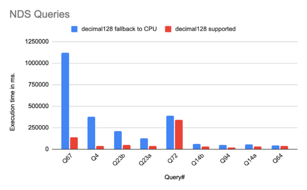
Preliminary runs of a subset of NDS queries demonstrate significant performance improvement due to decimal128 support, as shown in the following graph. These were run on a cluster of eight nodes each with one A100 GPU and 1024 CPU cores, running executors with 16 cores on spark 3.1.1. Each executor uses 240GiB in memory. The queries show excellent speedup of nearly 8x, which can be attributed to operations that were previously falling back to the CPU now running on the GPU, thereby avoiding row-to-column and column-to-row transitions and other associated overheads. On average the end-to-end run time of all the NDS queries shows 2x improvement. This is (hopefully) just the beginning!
Figure 2: Performance evaluation of a subset of NDS queries.
With the 21.12 release of the RAPIDS plug-in for Spark, decimal128 support is available for the majority of operators. Some special handling of overflow conditions to maintain result compatibility between CPU and GPU is necessary. The ultimate goal of this effort is to allow retail and financial queries to fully benefit from GPU acceleration through the RAPIDS for Spark Plugin.
Summary
fixed_point types in RAPIDS libcudf, the addition of DecimalType, and decimal128 support for the RAPIDS plug-in for Spark enable exciting use cases that were previously only possible on the CPU now to be run on the GPU. If you want to get started with RAPIDS libcudf or the RAPIDS plug-in for Spark, you can follow the links below:
Who says you have to put your play on pause just because you’re not at your PC? This GFN Thursday takes a look at how GeForce NOW makes PC gaming possible on Android and iOS mobile devices to support gamers on the go. This week also comes with sweet in-game rewards for members playing Eternal Read article >
Researchers use advanced remote sensing and machine-learning algorithms to quickly monitor crop nitrogen levels, central to informing sustainable agriculture.
Powerful airborne sensors could be key in helping farmers sustainably manage maize across the US Corn Belt, according to a University of Illinois research team. The study, which employs remote sensors combined with newly developed deep learning models, gives an accurate and speedy prediction of crop nitrogen, chlorophyll, and photosynthetic capacity.
Published in the International Journal of Applied Earth Observation and Geoinformation, the work could guide farmer management practices, helping reduce fertilizer use, boost food production, and alleviate environmental damage across the region.
“Compared to the conventional approaches of leaf tissue analysis, remote sensing provides much faster and more cost-effective approaches to monitor crop nutrients. The timely and high-resolution crop nitrogen information will be very helpful to growers to diagnose crop growth and guide adaptive management,” said lead author Sheng Wang, a research scientist and assistant professor at the University of Illinois Urbana-Champaign.
Producing about 75% of corn in the US and 30% globally, the Corn Belt plays a major role in food production. Extending from Indiana to Nebraska, the region yields 20 times more than it did in the 1880s, thanks to improved farming, corn breeding, new technologies, and fertilizers.
Farmers rely on nitrogen-based fertilizers to boost photosynthesis, crop yields, and biomass for bioenergy crops. However, excessive application degrades soil, pollutes water sources, and contributes to global warming—nitrogen represents one of the largest sources of greenhouse gas emissions in agriculture.
Accurately measuring nitrogen levels in crops could help farmers avoid over application, but manually conducting surveys is time-consuming and labor-intensive.
“Precision agriculture that relies on advanced sensing technologies and airborne satellite platforms to monitor crops could be the solution,” said project lead Kaiyu Guan, the Blue Waters Associate Professor at the University of Illinois Urbana-Champaign.
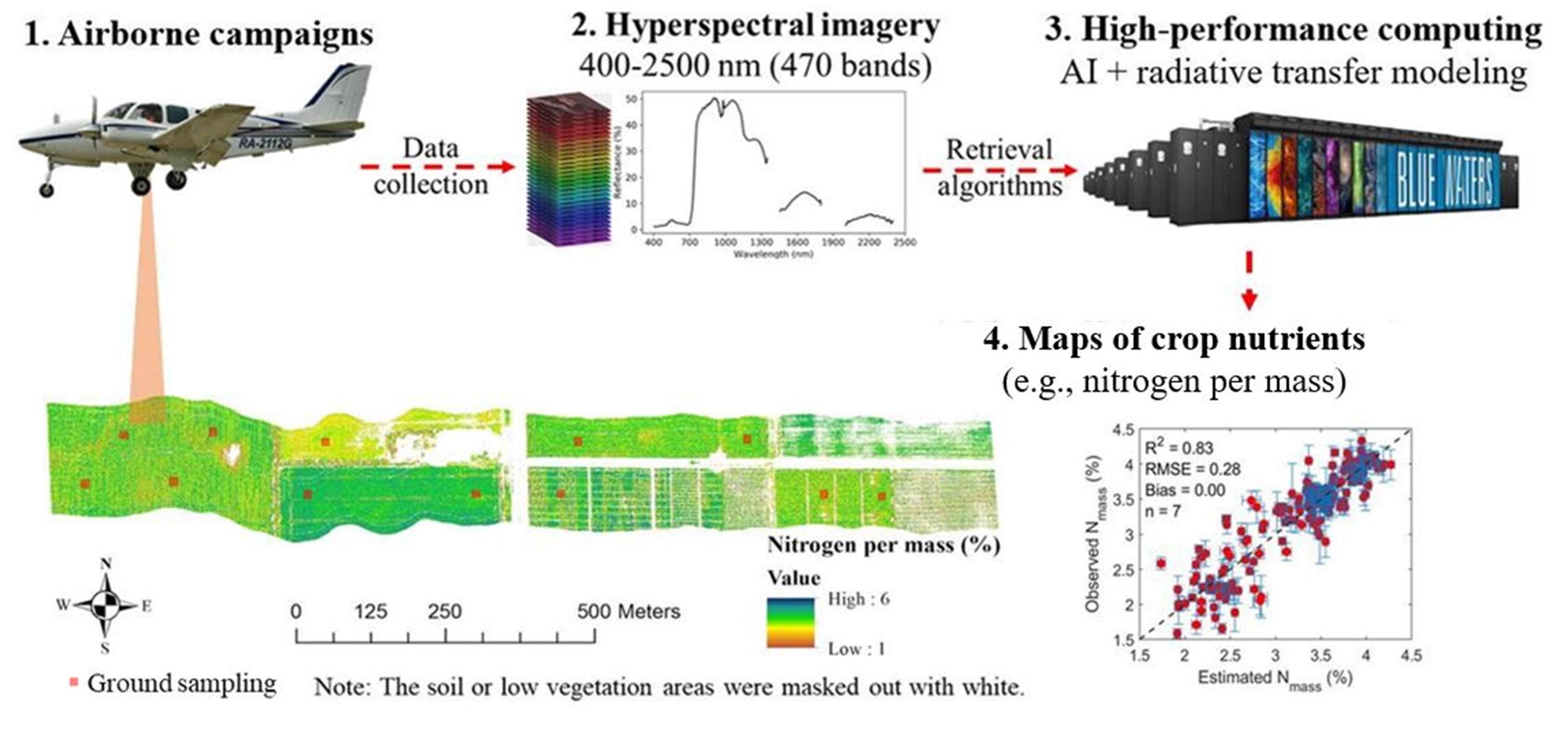
Up until now, there has not been a reliable method for quickly monitoring leaf nitrogen levels over the course of a growing season. Using hyperspectral imaging and machine-learning models, the team proposed a hybrid approach to address these limitations.
Hyperspectral imaging—an expanding area of remote sensing—uses a spectrometer that breaks down a pixel into hundreds of images at different wavelengths, providing more information on the captured image.
Equipped with a highly sensitive hyperspectral sensor, the researchers conducted plane surveys over an experimental field in Illinois, collecting crop reflectance data. Plant chemical composition, such as nitrogen and chlorophyll influences reflection, which the sensors can detect even in subtle wavelength changes of just 3 to 5 nanometers.
Figure 1. An illustrative summary of methods for the study, “Airborne hyperspectral imaging of nitrogen deficiency on crop traits and yield of maize by machine learning and radiative transfer modeling.” Courtesy of Sheng Wang.
Using Radiative Transfer Modeling and a data-driven Partial-Least Squares Regression (PLSR) approach, the team developed deep learning models to predict crop traits based on the airborne reflectance data. According to the study, PLSR requires a relatively small size of label data for model training.
The researchers trained their deep learning models using cuDNN and NVIDIA V100 GPUs to predict crop nitrogen, chlorophyll, and photosynthetic capacity at both leaf and canopy levels.
Testing the algorithms against ground-truth data, the models were about 85% accurate. The technique is fast, scanning fields in just a few seconds per acre. According to Wang, such technology can be very helpful to diagnose crop nitrogen status and yield potential.
The ultimate goal of the work is to use satellite imagery for large-scale nitrogen monitoring across every field in the US Corn Belt and beyond.
“We hope this technology can provide stakeholders timely information and advance growers’ management practices for sustainable agricultural practices,” Guan said.
Read the study in the International Journal of Applied Earth Observation and Geoinformation. >> Read more. >>
Hi all,I have successfully used the Object Detection API to train a model and am now trying to obtain a list of the class name and scores for the objects detected. Here is the code:
EDIT: Scores will not be required if the final output would only be a single class name. Thank you.
While this launches the cv2 display window successfully, I have been unable to find any workable solution to get class name or the score. Generally, I was unable to find no viable solutions at all, barring this one, but after trying the solution it has proven to unsuccessful too.
I hope that I can be pointed towards a tutorial for this, but any help/thoughts will be greatly appreciated.
Posted by Zizhao Zhang, Software Engineer, Google Cloud
In visual understanding, the Visual Transformer (ViT) and its variants have received significant attention recently due to their superior performance on many core visual applications, such as image classification, object detection, and video understanding. The core idea of ViT is to utilize the power of self-attention layers to learn global relationships between small patches of images. However, the number of connections between patches increases quadratically with image size. Such a design has been observed to be data inefficient — although the original ViT can perform better than convolutional networks with hundreds of millions of images for pre-training, such a data requirement is not always practical, and it still underperforms compared to convolutional networks when given less data. Many are exploring to find more suitable architectural re-designs that can learn visual representations effectively, such as by adding convolutional layers and building hierarchical structures with local self-attention.
The principle of hierarchical structure is one of the core ideas in vision models, where bottom layers learn more local object structures on the high-dimensional pixel space and top layers learn more abstracted and high-level knowledge at low-dimensional feature space. Existing ViT-based methods focus on designing a variety of modifications inside self-attention layers to achieve such a hierarchy, but while these offer promising performance improvements, they often require substantial architectural re-designs. Moreover, these approaches lack an interpretable design, so it is difficult to explain the inner-workings of trained models.
To address these challenges, in “Nested Hierarchical Transformer: Towards Accurate, Data-Efficient and Interpretable Visual Understanding”, we present a rethinking of existing hierarchical structure–driven designs, and provide a novel and orthogonal approach to significantly simplify them. The central idea of this work is to decouple feature learning and feature abstraction (pooling) components: nested transformer layers encode visual knowledge of image patches separately, and then the processed information is aggregated. This process is repeated in a hierarchical manner, resulting in a pyramid network structure. The resulting architecture achieves competitive results on ImageNet and outperforms results on data-efficient benchmarks. We have shown such a design can meaningfully improve data efficiency with faster convergence and provide valuable interpretability benefits. Moreover, we introduce GradCAT, a new technique for interpreting the decision process of a trained model at inference time.
Architecture Design The overall architecture is simple to implement by adding just a few lines of Python code to the source code of the original ViT. The original ViT architecture divides an input image into small patches, projects pixels of each patch to a vector with predefined dimension, and then feeds the sequences of all vectors to the overall ViT architecture containing multiple stacked identical transformer layers. While every layer in ViT processes information of the whole image, with this new method, stacked transformer layers are used to process only a region (i.e., block) of the image containing a few spatially adjacent image patches. This step is independent for each block and is also where feature learning occurs. Finally, a new computational layer called block aggregation then combines all of the spatially adjacent blocks. After each block aggregation, the features corresponding to four spatially adjacent blocks are fed to another module with a stack of transformer layers, which then process those four blocks jointly. This design naturally builds a pyramid hierarchical structure of the network, where bottom layers can focus on local features (such as textures) and upper layers focus on global features (such as object shape) at reduced dimensionality thanks to the block aggregation.
A visualization of the network processing an image: Given an input image, the network first partitions images into blocks, where each block contains 4 image patches. Image patches in every block are linearly projected as vectors and processed by a stack of identical transformer layers. Then the proposed block aggregation layer aggregates information from each block and reduces its spatial size by 4 times. The number of blocks is reduced to 1 at the top hierarchy and classification is conducted after the output of it.
Interpretability This architecture has a non-overlapping information processing mechanism, independent at every node. This design resembles a decision tree-like structure, which manifests unique interpretability capabilities because every tree node contains independent information of an image block that is being received by its parent nodes. We can trace the information flow through the nodes to understand the importance of each feature. In addition, our hierarchical structure retains the spatial structure of images throughout the network, leading to learned spatial feature maps that are effective for interpretation. Below we showcase two kinds of visual interpretability.
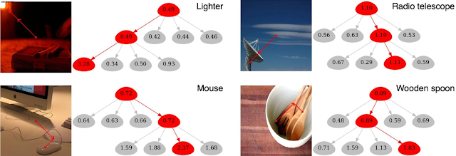
First, we present a method to interpret the trained model on test images, called gradient-based class-aware tree-traversal (GradCAT). GradCAT traces the feature importance of each block (a tree node) from top to bottom of the hierarchy structure. The main idea is to find the most valuable traversal from the root node at the top layer to a child node at the bottom layer that contributes the most to the classification outcomes. Since each node processes information from a certain region of the image, such traversal can be easily mapped to the image space for interpretation (as shown by the overlaid dots and lines in the image below).
The following is an example of the model’s top-4 predictions and corresponding interpretability results on the left input image (containing 4 animals). As shown below, GradCAT highlights the decision path along the hierarchical structure as well as the corresponding visual cues in local image regions on the images.
Given the left input image (containing four objects), the figure visualizes the interpretability results of the top-4 prediction classes. The traversal locates the model decision path along the tree and simultaneously locates the corresponding image patch (shown by the dotted line on images) that has the highest impact to the predicted target class.
Moreover, the following figures visualize results on the ImageNet validation set and show how this approach enables some intuitive observations. For instance, the example of the lighter below (upper left panel) is particularly interesting because the ground truth class — lighter/matchstick — actually defines the bottom-right matchstick object, while the most salient visual features (with the highest node values) are actually from the upper-left red light, which conceptually shares visual cues with a lighter. This can also be seen from the overlaid red lines, which indicate the image patches with the highest impact on the prediction. Thus, although the visual cue is a mistake, the output prediction is correct. In addition, the four child nodes of the wooden spoon below have similar feature importance values (see numbers visualized in the nodes; higher indicates more importance), which is because the wooden texture of the table is similar to that of the spoon.
Visualization of the results obtained by the proposed GradCAT. Images are from the ImageNet validation dataset.
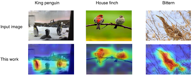
Second, different from the original ViT, our hierarchical architecture retains spatial relationships in learned representations. The top layers output low-resolution features maps of input images, enabling the model to easily perform attention-based interpretation by applying Class Attention Map (CAM) on the learned representations at the top hierarchical level. This enables high-quality weakly-supervised object localization with just image-level labels. See the following figure for examples.
Visualization of CAM-based attention results. Warmer colors indicate higher attention. Images are from the ImageNet validation dataset.
Convergence Advantages With this design, feature learning only happens at local regions independently, and feature abstraction happens inside the aggregation function. This design and simple implementation is general enough for other types of visual understanding tasks beyond classification. It also improves the model convergence speed greatly, significantly reducing the training time to reach the desired maximum accuracy.
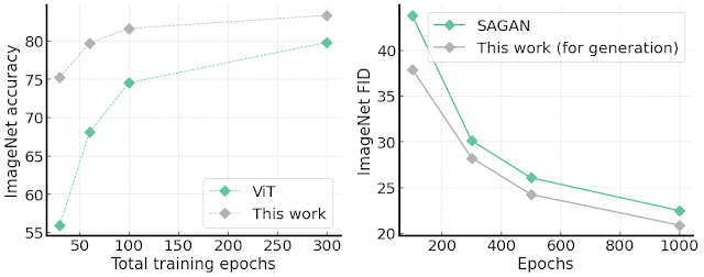
We validate this advantage in two ways. First, we compare the ViT structure on the ImageNet accuracy with a different number of total training epochs. The results are shown on the left side of the figure below, demonstrating much faster convergence than the original ViT, e.g., around 20% improvement in accuracy over ViT with 30 total training epochs.
Second, we modify the architecture to conduct unconditional image generation tasks, since training ViT-based models for image generation tasks is challenging due to convergence and speed issues. Creating such a generator is straightforward by transposing the proposed architecture: the input is an embedding vector, the output is a full image in RGB channels, and the block aggregation is replaced by a block de-aggregation component supported by Pixel Shuffling. Surprisingly, we find our generator is easy to train and demonstrates faster convergence speed, as well as better FID score (which measures how similar generated images are to real ones), than the capacity-comparable SAGAN.
Left: ImageNet accuracy given different number of total training epochs compared with standard ViT architecture. Right: ImageNet 64×64 image generation FID scores (lower is better) with single 1000-epoch training. On both tasks, our method shows better convergence speed.
Conclusion In this work we demonstrate the simple idea that decoupled feature learning and feature information extraction in this nested hierarchy design leads to better feature interpretability through a new gradient-based class-aware tree traversal method. Moreover, the architecture improves convergence on not only classification tasks but also image generation tasks. The proposed idea is focusing on aggregation function and thereby is orthogonal to advanced architecture design for self-attention. We hope this new research encourages future architecture designers to explore more interpretable and data-efficient ViT-based models for visual understanding, like the adoption of this work for high-resolution image generation. We have also released the source code for the image classification portion of this work.
Acknowledgements We gratefully acknowledge the contributions of other co-authors, including Han Zhang, Long Zhao, Ting Chen, Sercan Arik, Tomas Pfister. We also thank Xiaohua Zhai, Jeremy Kubica, Kihyuk Sohn, and Madeleine Udell for the valuable feedback of the work.
After meeting at an entrepreneur matchmaking event, Ulrik Hansen and Eric Landau teamed up to parlay their experience in financial trading systems into a platform for faster data labeling. In 2020, the pair of finance industry veterans founded Encord to adapt micromodels typical in finance to automated data annotation. Micromodels are neural networks that require Read article >


 Sharpen your conversational AI, vehicle routing, or CUDA Python skills; learn how Metropolis boosts go-to-market efforts; find solutions for AI inference deployment.
 This post details CUDA’s new int128 support and how to implement decimal fixed-point arithmetic on top of it.


 Researchers use advanced remote sensing and machine-learning algorithms to quickly monitor crop nitrogen levels, central to informing sustainable agriculture.