This year, Microsoft’s free Game Stack Live event (April 20-21), starting at 8am PDT, will offer a wide range of can’t-miss sessions for game developers, in categories that include Graphics, System & Tools, Production & Publishing, Accessibility & Inclusion, Audio, Multiplayer, and Community Connections.
This year, Microsoft’s free Game Stack Live event (April 20-21), starting at 8am PDT, will offer a wide range of can’t-miss sessions for game developers, in categories that include Graphics, System & Tools, Production & Publishing, Accessibility & Inclusion, Audio, Multiplayer, and Community Connections.
NVIDIA will be participating with two talks:
Introduction to Real-Time Ray Tracing with Minecraft
This talk is aimed at graphics engineers that have little or no experience with ray tracing. It serves as a gentle introduction to many topics, including “What is ray tracing?”, “How many rays do you need to make an image?”, “The importance of [importance] sampling. (And more importantly, what is importance sampling?)”, “Denoising”, “The problem with small bright things”. Along the way, you will learn about specific implementation details from Minecraft.
RTXDI: Details on Achieving Real-time Performance
RTXDI offers realistic lighting of dynamic scenes that require computing shadows from millions of area lights. Until now, this has not been possible in video games. Traditionally, game developers have baked most lighting and supported a small number of “hero” lights that are computed at runtime. This talk gives an overview of RTXDI and offers a deep dive into previously undisclosed details that enable high performance.
This post was originally published on the Mellanox blog in April 2020. People generally assume that faster network interconnects maximize endpoint performance. In this post, I examine the key factors and considerations when choosing the right speed for your leaf-spine data center network. To establish a common ground and terminology, Table 1 lists the five … Continued
This post was originally published on the Mellanox blog in April 2020.
People generally assume that faster network interconnects maximize endpoint performance. In this post, I examine the key factors and considerations when choosing the right speed for your leaf-spine data center network.
To establish a common ground and terminology, Table 1 lists the five building blocks of a standard leaf-spine networking infrastructure.
Building block
Role
Network interface card (NIC)
A gateway between the server (compute resource) and network.
Leaf switch/top-of-rack switch
The first connection from the NIC to the rest of the network.
Spine switch
The “highway” junctions, responsible for the east-west traffic. Its port capacity determines the number of required racks.
Cable
Connects the different devices in the network.
Optic transceiver
Allows longer distances of connectivity (above a few meters) between a leaf-to-spine switch by modulating the data into light that traverses the optic cable.
Table 1. Five building blocks of a standard leaf-spine networking infrastructure.
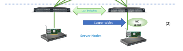
I start by reviewing the trends in 2020 for data center leaf-spine networks deployments and describing the main ecosystem that lies behind it all. Figure 1 shows an overview of leaf-spine network connectivity. It is divided into two main connectivity parts, each of which takes different factors into consideration when picking the deployment rate:
Switch-to-switch (applies also when using a level of super-spine)
NIC-to-switch
Figure 1. Leaf-spine network connectivity.
Together these parts comprise an ecosystem, which I now analyze in depth.
Switch-to-switch speed dynamics
New leaf-spine data center deployments in 2020 evolve around four IEEE approved speeds: 40, 100, 200, and 400GbE. There are different combinations of supported switches per speed. For example, constructing a network of 400GbE leaf-spine connectivity requires the network owner to pick switches and cables that can support those rates.
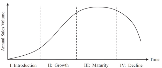
Like every other product in the world, each speed generation demonstrates a unique product life cycle (PLC), while each stage comes with its own attributes.
Figure 2. A typical product life cycle.
Introduction—Product adoption is concentrated within a small group of innovators who are neither afraid to take risks nor suffer from birth pangs. In networking, these are usually the networking giants (also known as hyperscalers).
Growth—Occurs as leaders and decision makers start adopting a new generation.
Maturity—Characterized by the adoption of products by more conservative customers.
Decline—A speed generation is used to connect legacy equipment.
The main questions that pop-up in my mind are, “Why do generations change?” and “What drives the ambition for faster switch-to-switch connectivity?” The answer for both is surprisingly simple: $MONEY$. When you constantly optimize your production process and, at the same time, allow bigger scale (bigger ASIC switching capacity), the result is lower connectivity costs.
This price reduction does not happen at once; it takes time to reach maturity. Hyperscalers can benefit from cost reduction even when a generation is in its Introduction stage, because being big allows them to get better prices (the economy of scale offers better buying power), often much lower than the manufacturer’s suggested retail price. In some sense, you could say that hyperscalers are paving the way for the rest of the market to use new generations.
Armed with this new knowledge, here’s some analysis.
Before focusing on the present, rewind a decade, back to 2010-11, when 10GbE was approaching maturity and the industry was hyped about transitioning from a 10 to 100GbE switch-to-switch speed. At the time, the 100GbE leaf-spine ecosystem had many caveats, including that 100GbE NRZ technology spine switches did not have the right radix for scale, providing only 12 ports of 100GbE in a spine switch, meaning only 12 racks could have been connected in a leaf-spine cluster.
Also, at the same time, 40GbE switch-to-switch connectivity started to gain traction even though it was slower, due to mature SerDes technology, a reliable ASIC process, better scale, and lower overall cost for most of the market.
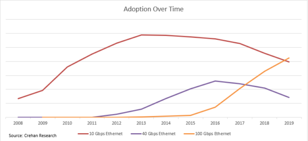
Put yourself in the shoes of a decision maker who needs to deploy a new cluster in 2011: what switch-to-switch speed would you pick? Hard dilemma, right? Fortunately, as it was a decade ago, we have since accumulated lots of data about what happened. Take a moment to analyze Figure 3. The 10/40GbE generation is a perfect example for a PLC curve.
Figure 3. Adoption over time.
Beginning in 2011 until 2015, most of the industry picked 40GbE as its leaf-spine network speed. When asked in retrospect about the benefits of 40GbE, businesses typically mention improved application performance and better ROI. Only at the end of 2015, roughly four years after the advent of 40GbE, did the 100GbE leaf-spine ecosystem begin its rise and be seen as reliable and cost-effective. Some deployments did benefit from 100GbE, since picking “the latest and the greatest” would fit some use cases, even at higher prices.
Fast forward to 2020
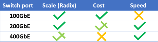
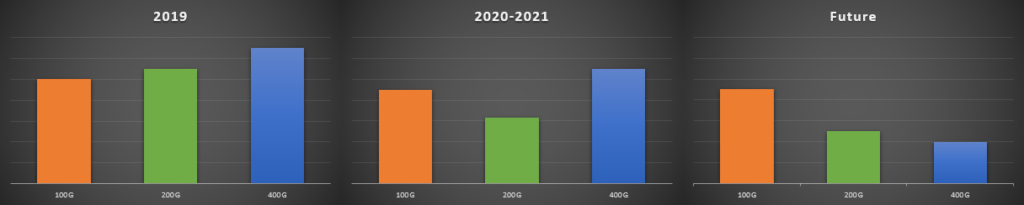
New data center deployments enjoy a set of wonderful new options of switch-to-switch rates to pick from, starting from 40GbE to 400GbE. Most of the current deployments are using 100GbE connections, which is mature at this point. With the continuous drive to lower costs, the demand for faster network speeds isn’t easing up, as newer technologies of 200GbE and 400GbE are deployed. Figure 4 presents the attributes currently associated with each switch-to-switch speed generation.
Figure 4. Attributes of switch-to-switch speed generation.
You can conclude that each generation has its own pros and cons and picking one should be based on your personal preferences. Now I explain the dynamics taking place in the data center speed ecosystem and try to answer which switch-to-switch speed generation fits you best: 100, 200, or 400GbE?
Dynamics between switch-to-switch speed and NIC-to-switch speed
As mentioned earlier, new switch-to-switch data center deployments in 2020 evolve around four IEEE approved speeds: 40, 100, 200, and 400GbE. Each one is at a different PLC stage (Table 2).
switch-to-switch speed
switch-to-switch generation stage (2020)
40GbE
Decline
100GbE
Maturity
200GbE
Growth
400GbE
Introduction (with several years to reach growth, according to past leaps and current market trends)
Table 2. Product life cycle stages.
Let me share with you the reasons I view the market in this way. To begin with, 400GbE is the current latest and greatest. No doubt, it will take a major part of deployments in the future by offering the fastest connectivity, with a projected lowest cost per GbE. However, at the present, it still has not reached the required maturity to gain the associated benefits of commoditization.
A small number of hyperscalers—known for innovation, compute-intense applications, engineering capabilities, and most importantly, enjoying the economy of scale—are deploying clusters at that speed. To mitigate technical issues with 400GbE native connections, some have shifted to 2x200GbE or pure 200GbE deployments. The reason is that with 200GbE leaf-spine connections, hyperscalers can rely on a more resilient infrastructure, leveraging both cheaper optics and switch radix that allows for scaling a fabric.
At present, non-hyperscalers trying to move to 400GbE switch-to-switch connectivity may come to realize that the cables and transceivers are still expensive and produced in low volumes. Moreover, the 7nm ASIC process for creating high-capacity switches is not optimized.
At the opposite side of the curve lies the 40GbE, which is a generation in decline. You should consider 40GbE if you are deploying a legacy cluster, with legacy equipment that cannot work at faster speeds.
Most of the market is not being caught up in the hype and doesn’t waste money on unnecessary bandwidth. It is focused on the 100GbE mature ecosystem. Because it exhibits textbook characteristics when it comes to cost reduction, market availability and reliability means that the 100GbE is not going away. It is here to stay.
This is a great opportunity to mention the other part of the story: the NIC-to-switch speed. At this point, it might seem that they co-exist orthogonally, but in fact they are entwined and affect one another.
Figure 5. NIC-to-switch and switch-to-switch affect each other.
Whether your application is in the field of intense compute, storage, or AI, the NIC is the heart of it. In practice, the NIC speed determines the optimal choice of the surrounding network infrastructure, as it connects your compute and storage to the network. When deciding the switch-to-switch speed to pick, also consider what kind of traffic, generated from the compute nodes, is going to run between the switches. Different applications have different traffic patterns. Nowadays, most of the traffic in a data center is east-west traffic, from one NIC to another.
To get the best application performance, opt for a leaf switch that has the appropriate blocking factor (optimally non-blocking at all) to avoid congestion, by deploying enough uplink and downlink ports.
Data center deployments frequently use NICs at one of the following speeds:
10GbE (NRZ)
25GbE (NRZ)
50GbE (PAM-4)
100GbE (PAM-4)
There are also 50GbE and 100GbE NRZ NICs, but they are less common.
This is where the complete ecosystem builds up, the point where switch-to-switch and NIC-to-switch complement each other. After reviewing dozens of different data center deployments, I noticed that there is a clear pattern when it comes to overall costs, regarding choosing a switch-to-switch speed when considering also the NIC-to-switch speed-of-choice. The math just works that way. There is an optimal point where a specific switch-to-switch speed generation allows the NIC-to-switch speed to maximize application performance, both in terms of bandwidth utilization and ROI.
Take into consideration the application, wanted blocking factor, and price per GbE. If your choice is based on the NIC speed, you would probably want to use the switch-to-switch speed, as shown in Table 3.
NIC port speed
Possible use case (2020)
Recommended switch-to-switch speed
100GbE PAM-4
Hyperscalers, innovators
200/400GbE
50GbE PAM-4
Hyperscalers, innovators, AI, advanced storage applications, public cloud
200/400GbE
25GbE NRZ
Enterprises, private cloud, HCI, edge
100GbE
10GbE NRZ
Legacy
40GbE
Table 3. Optimal NIC-to-switch speed. 50/100GbE NRZ act the same as 25GbE NRZ economically.
Of course, other combinations might be better, depending on the prices you get from your vendor, but on average, this is how I view the market.
Here are some important takeaways:
Lower the cost per GbE, the switch-to-switch speed is always increasing. A new generation is introduced every several years.
When picking according to the NIC-to-switch speed, consider the projected traffic patterns and the necessary blocking pattern from the leaf-switch.
Data center maturity is determined from the maturity of both switch-to-switch and NIC-to-switch speeds.
Along comes 200GbE
If you’ve made it this far, then you must have realized that 200GbE leaf-spine speed is also an option to consider.
In December 2017, the IEEE approved a standard that contains the specifications for 200 and 400GbE. As discussed earlier, a small number of hyperscalers are upgrading their deployment from 100GbE to 400GbE directly. Practically speaking, the industry acknowledged that the 200GbE can serve as an intermediate step, like the transition between 10 to 100GbE, in which 40GbE served as an intermediate step.
So, what’s in it for you?
200GbE switch-to-switch deployments enjoy a comprehensive set of benefits:
Increased ROI by doubling the bandwidth using a ready-to-deploy ecosystem (NIC, Switch, Cable & Transceiver) with an economical premium over 100GbE. The cost analysis just makes sense, providing the lowest price per GbE (Figure 6).
Figure 6. Past and expected price per GbE using different switch-to-switch connectivity.
The next generation of switch and NIC ASICs, with an improved feature set, including enhanced telemetry.
A reduced cable footprint, to avoid signal integrity problems and cable crosstalk in a high-density front panel 100GbE switch compared to half the number of ports in a 200GbE switch.
200G is a native rate of InfiniBand (IB). Leading the IB market in supplying switches, NICs and cables/transceivers, NVIDIA has proven this technology mature, by providing over 1M ports of 200G, reaching economy of scale and optimizing price. The NVIDIA 200GbE supporting devices (NICs, cables, and transceivers) are shared between IB and Ethernet.
In preparation for the 200/400GbE era, NVIDIA has optimized its 200GbE switch portfolio. It allows the fabric to scale the radix with better ROI than 400GbE, by using a 64×200(12.8Tbps) spine and 12×200+48×50(6.4Tbps) as a non-blocking leaf switch.
When you consider the competition, NVIDIA offers an optimized non-blocking leaf switch (top-of-rack) for 50 G PAM-4 NICs.
NVIDIA Spectrum-2 based platforms provide a capacity of 6.4 Tb, 50 G PAM-4 SerDes and a feature set that complies with the virtualized data center environment.
Using a competitor’s 12.8TbE switch as a leaf switch is just overkill for today’s deployments because the majority of top-of-rack switches have 48 downlink ports of 50GbE. By doing the math to get to a non-blocking ratio, the switches need 6 ports of 400 or 12 ports of 200GbE, resulting in a total of 4.8TbE. There is no added value to paying for unused switching capacity.
By the way, NVIDIA offers a 200GbE development kit for people who want to take the SN3700 Ethernet switch for a test drive.
Summary
Deploying or upgrading a data center in 2020? Make sure to take into consideration the following:
The market is dynamic, and past trends may assist you in predicting future ones
Select your switch-to-switch and NIC-to-switch speed according to your requirements
200GbE holds massive benefits
Disagree with the need for 200GbE, or anything else in this post? Feel free to reach out to me. I would love to have a discussion with you.
What can I do, to get Tensorflow to finally calcuate the result. I have trouble to understand EagerMode and GraphMode. Maybe a good Youtube resource may also help.
Over the past couple of years, NVIDIA and NASA have been working closely on accelerating data science workflows using RAPIDS and integrating these GPU-accelerated libraries with scientific use cases. In this blog, we’ll share some of the results from an atmospheric science use case, and code snippets to port existing CPU workflows to RAPIDS on … Continued
Over the past couple of years, NVIDIA and NASA have been working closely on accelerating data science workflows using RAPIDS and integrating these GPU-accelerated libraries with scientific use cases. In this blog, we’ll share some of the results from an atmospheric science use case, and code snippets to port existing CPU workflows to RAPIDS on NVIDIA GPUs.
Accelerated Simulation of Air Pollution from Christoph Keller
One example science use case from NASA Goddard simulates chemical compositions of the atmosphere to monitor, forecast, and better understand the impact of air pollution on the environment, vegetation, and human health. Christoph Keller, a research scientist at the NASA Global Modeling and Assimilation Office, is exploring alternative approaches based on machine learning models to simulate the chemical transformation of air pollution in the atmosphere. Doing such calculations with a numerical model is computationally expensive, which limits the use of comprehensive air quality models for real-time applications such as air quality forecasting. For instance, the NASA GEOS composition forecast model GEOS-CF, which simulates the distribution of 250 chemical species in the Earth atmosphere in near real-time, needs to be run on more than 3000 CPUs and more than 50% of the required compute cost is related to the simulation of chemical interactions between these species.
Figure 1: Simulation of Atmospheric Chemistry, 56 million grid cells (25×25 km2, 72 levels) and 250 chemical species.
We were able to accelerate the simulation of atmospheric chemistry in the NASA GEOS Model with GEOS-Chem chemistry more than 10-fold by replacing the default numerical chemical solver in the model with XGBoost emulators. To train these gradients boosted decision tree models, we produced a dataset using hourly output from the original GEOS model with GEOS-Chem chemistry. The input dataset contains 126 key physical and chemical parameters such as air pollution concentrations, temperature, humidity, and sun intensity. Based on these inputs, the XGBoost model is trained to predict the chemical formation (or destruction) of an air pollutant under the given atmospheric conditions. Separate emulators are trained for individual chemicals.
To make sure that the emulators are accurate for the wide range of atmospheric conditions found in the real world, the training data needs to capture all geographic locations and annual seasons. This results in very large training datasets – quickly spanning 100s of millions of data points, making it slow to train. Using RAPIDS Dask-cuDF (GPU-accelerated dataframes) and training XGBoost on an NVIDIA DGX-1 with 8 V100 GPUs, we are able to achieve 50x overall speedup compared to Dual 20-Core Intel Xeon E5-2698 CPUs on the same node.
An example of this is given in the gc-xgb repo sample code, showcasing the creation of an emulator for the chemical compound ozone (O3), a key air pollutant and climate gas. For demonstration purposes, a comparatively small training data set spanning 466,830 samples is used. Each sample contains up to 126 non-zero features, and the full size of the training data contains 58,038,743 entries. In the provided example, the training data – along with the corresponding labels – is loaded from a pre-generated txt file in svmlight / libsvm format, available in the GMAO code repo:
Loading the training data from a pre-generated text file, as shown in the example here, sidesteps the data preparation process whereby the 4-dimensional model data (latitude x longitude x altitude x time) as generated by the GEOS model (in netCDF format) are being read, subsampled and flattened.
The loaded training data can directly be used to train an XGBoost model:
Setting the tree_method to ‘gpu_hist’ instead of ‘hist’ performs the training on GPUs instead of CPUs, highlighting a significant speed-up in training time even for the comparatively small sample training data used in this example. This difference is exacerbated on the much larger data sets needed for developing emulators suitable for actual use in the GEOS model. Since our application requires training of dozens of ML emulators – ideally on a recurring basis as new model data is produced – the much shorter training time on RAPIDS is critical and ensures a short enough model development cycle.
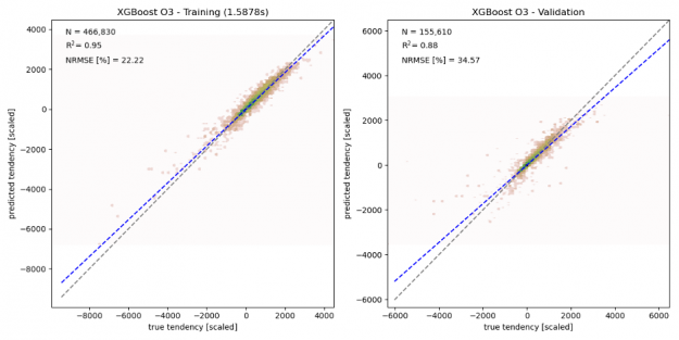
As shown in the figure below, the chemical tendencies of ozone (i.e., the change in ozone concentration due to atmospheric chemistry) predicted by the gradient boosted decision tree model shows good agreement with the true chemical tendencies simulated by the numerical model. Given the relatively small training sample size (466,830 samples), the here trained model shows some signs of overfitting, with the correlation coefficient R2 dropping from 0.95 for the training data to 0.88 in the validation data, and the normalized root means square error (NRMSE) increasing from 22% to 35%. This indicates that larger training samples are needed to ensure that the training dataset captures all chemical environments.
Figure 2: Simulation of Atmospheric Chemistry, 56 million grid cells (25×25 km2, 72 levels) and 250 chemical species.
In order to deploy the XGBoost emulator in the GEOS model as a replacement to the GEOS-Chem chemical solver, the XGBoost algorithm needs to be called from within the GEOS modeling system, which is written in Fortran. To do so, the trained XGBoost model is saved to disk so that it can then be read (and evoked) from a Fortran model by leveraging XGBoost’s C API (The XGBoost interface for Fortran can be found in the fortran2xgb GitHub repo.
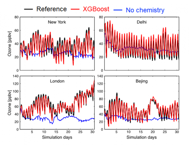
As shown in the figure below, running the GEOS model with atmospheric chemistry emulated by XGBoost produces surface ozone concentrations that are similar to the numerical solution (red vs. black line). The blue line shows a simulation using a model with no chemistry, highlighting the critical role of atmospheric chemistry for surface ozone.
GEOS model simulations using XGBoost emulators instead of the GEOS-Chem chemical solver have the potential to be 20-50% faster than the reference simulation, depending on the model configuration (such as horizontal and temporal resolution). By offering a much faster calculation of atmospheric chemistry, these ML emulators open the door for a range of new applications, such as probabilistic air quality forecasts or a better combination of atmospheric observations and model simulations. Further improvements to the ML emulators can be achieved through mass balance considerations and by accounting for error correlations, tasks that Christoph and colleagues are currently working on.
Figure 3: Surface concentrations of O3 at four locations for the GEOS-Chem reference (black), XGBoost model (red) and simulation with no chemistry (blue), indicate that these regions are well reproduced by the XGB model and capture the concentration patterns.
In the next blog, we’ll talk about another application leveraging XGBoost and RAPIDS for live monitoring of air quality across the globe during the COVID-19 pandemic.
Keller, C. A. and Evans, M. J.: Application of random forest regression to the calculation of gas-phase chemistry within the GEOS-Chem chemistry model v10, Geosci. Model Dev., 12, 1209–1225, https://doi.org/10.5194/gmd-12-1209-2019, 2019.
My dataset uses tf.train.SequenceExample, which contains a sequence of N elements, and this N by definition can vary from one sequence to another. I want to select M, which is fixed for all sequences, elements uniformly from the N elements. For example, if the sequence has N=10 elements, then for M = 2 I want to select index=0, index=5 elements. M will always be smaller than any N in the dataset.
Now the issue is, when dataset iterator calls parser function through the ‘map’ method it is executed in the ‘graph’ mode and axis dimension corresponding to ‘N’ is ‘None’. So, I can’t iterate on that axis to find the value of N.
I resolved this issue by using tf.py_function, but it is 10X slower. I tried using tf.data.AUTOTUNE in num_parallel_calls and also in prefetch, and also set deterministic=False, But performance is still 10X slower.
The network compiles and trains, but I get the following warning while training:
WARNING:tensorflow:Model was constructed with shape (None, 1061, 4) for input KerasTensor(type_spec=TensorSpec(shape=(None, 1061, 4), dtype=tf.float32, name=’input_1′), name=’input_1′, description=”created by layer ‘input_1′”), but it was called on an input with incompatible shape (None, 4).
I double-checked my inputs, and indeed there are 7 arrays of shape (1061, 4). What am I doing wrong here?
It’s Thursday, which means it’s GFN Thursday — when GeForce NOW members can learn what new games and updates are streaming from the cloud. This GFN Thursday, we’re checking in on one of our favorite gaming franchises, the Stronghold series from Firefly Studios. We’re also sharing some sales Firefly is running on the Stronghold franchise. Read article >
Shalini De Mello, a principal research scientist at NVIDIA who’s made her mark inventing computer vision technology that contributes to driver safety, finished 2020 with a bang — presenting two posters at the prestigious NeurIPS conference in December. A 10-year NVIDIA veteran, De Mello works on self-supervised and few-shot learning, 3D reconstruction, viewpoint estimation and Read article >
Posted by Negar Saei, Program Manager, University Relations
In March 2020 we introduced the Research Scholar Program, an effort focused on developing collaborations with new professors and encouraging the formation of long-term relationships with the academic community. In November we opened the inaugural call for proposals for this program, which was received with enthusiastic interest from faculty who are working on cutting edge research across many research areas in computer science, including machine learning, human computer interaction, health research, systems and more.
Today, we are pleased to announce that in this first year of the program we have granted 77 awards, which included 86 principal investigators representing 15+ countries and over 50 universities. Of the 86 award recipients, 43% identify as an historically marginalized group within technology. Please see the full list of 2021 recipients on our web page, as well as in the list below.
We offer our congratulations to this year’s recipients, and look forward to seeing what they achieve!
Algorithms and Optimization Alexandros Psomas, Purdue University Auction Theory Beyond Independent, Quasi-Linear Bidders Julian Shun, Massachusetts Institute of Technology Scalable Parallel Subgraph Finding and Peeling Algorithms Mary Wootters, Stanford University The Role of Redundancy in Algorithm Design Pravesh K. Kothari, Carnegie Mellon University Efficient Algorithms for Robust Machine Learning Sepehr Assadi, Rutgers University Graph Clustering at Scale via Improved Massively Parallel Algorithms
Augmented Reality and Virtual Reality Srinath Sridhar, Brown University Perception and Generation of Interactive Objects
Geo Miriam E. Marlier, University of California, Los Angeles Mapping California’s Compound Climate Hazards in Google Earth Engine Suining He, The University of Connecticut Fairness-Aware and Cross-Modality Traffic Learning and Predictive Modeling for Urban Smart Mobility Systems
Human Computer Interaction Arvind Satyanarayan, Massachusetts Institute of Technology Generating Semantically Rich Natural Language Captions for Data Visualizations to Promote Accessibility Dina EL-Zanfaly, Carnegie Mellon University In-the-making: An intelligence mediated collaboration system for creative practices Katharina Reinecke, University of Washington Providing Science-Backed Answers to Health-related Questions in Google Search Misha Sra, University of California, Santa Barbara Hands-free Game Controller for Quadriplegic Individuals Mohsen Mosleh, University of Exeter Business School Effective Strategies to Debunk False Claims on Social Media: A large-scale digital field experiments approach Tanushree Mitra, University of Washington Supporting Scalable Value-Sensitive Fact-Checking through Human-AI Intelligence
Health Research Catarina Barata, Instituto Superior Técnico, Universidade de Lisboa DeepMutation – A CNN Model To Predict Genetic Mutations In Melanoma Patients Emma Pierson, Cornell Tech, the Jacobs Institute, Technion-Israel Institute of Technology, and Cornell University Using cell phone mobility data to reduce inequality and improve public health Jasmine Jones, Berea College Reachout: Co-Designing Social Connection Technologies for Isolated Young Adults Mojtaba Golzan, University of Technology Sydney, Jack Phu, University of New South Wales Autonomous Grading of Dynamic Blood Vessel Markers in the Eye using Deep Learning Serena Yeung, Stanford University Artificial Intelligence Analysis of Surgical Technique in the Operating Room
Machine Learning and data mining Aravindan Vijayaraghavan, Northwestern University, Sivaraman Balakrishnan, Carnegie Mellon University Principled Approaches for Learning with Test-time Robustness Cho-Jui Hsieh, University of California, Los Angeles Scalability and Tunability for Neural Network Optimizers Golnoosh Farnadi, University of Montreal, HEC Montreal/MILA Addressing Algorithmic Fairness in Decision-focused Deep Learning Harrie Oosterhuis, Radboud University Search and Recommendation Systems that Learn from Diverse User Preferences Jimmy Ba, University of Toronto Model-based Reinforcement Learning with Causal World Models Nadav Cohen, Tel-Aviv University A Dynamical Theory of Deep Learning Nihar Shah, Carnegie Mellon University Addressing Unfairness in Distributed Human Decisions Nima Fazeli, University of Michigan Semi-Implicit Methods for Deformable Object Manipulation Qingyao Ai, University of Utah Metric-agnostic Ranking Optimization Stefanie Jegelka, Massachusetts Institute of Technology Generalization of Graph Neural Networks under Distribution Shifts Virginia Smith, Carnegie Mellon University A Multi-Task Approach for Trustworthy Federated Learning
Mobile Aruna Balasubramanian, State University of New York – Stony Brook AccessWear: Ubiquitous Accessibility using Wearables Tingjun Chen, Duke University Machine Learning- and Optical-enabled Mobile Millimeter-Wave Networks
Machine Perception Amir Patel, University of Cape Town WildPose: 3D Animal Biomechanics in the Field using Multi-Sensor Data Fusion Angjoo Kanazawa, University of California, Berkeley Practical Volumetric Capture of People and Scenes Emanuele Rodolà, Sapienza University of Rome Fair Geometry: Toward Algorithmic Debiasing in Geometric Deep Learning Minchen Wei, The Hong Kong Polytechnic University Accurate Capture of Perceived Object Colors for Smart Phone Cameras Mohsen Ali, Information Technology University of the Punjab, Pakistan, Izza Aftab, Information Technology University of the Punjab, Pakistan Is Economics From Afar Domain Generalizable? Vineeth N Balasubramanian, Indian Institute of Technology Hyderabad Bridging Perspectives of Explainability and Adversarial Robustness Xin Yu, University of Technology Sydney, Linchao Zhu, University of Technology Sydney Sign Language Translation in the Wild
Networking Aurojit Panda, New York University Bertha: Network APIs for the Programmable Network Era Cristina Klippel Dominicini, Instituto Federal do Espirito Santo Polynomial Key-based Architecture for Source Routing in Network Fabrics Noa Zilberman, University of Oxford Exposing Vulnerabilities in Programmable Network Devices Rachit Agarwal, Cornell University Designing Datacenter Transport for Terabit Ethernet
Natural Language Processing Danqi Chen, Princeton University Improving Training and Inference Efficiency of NLP Models Derry Tanti Wijaya, Boston University, Anietie Andy, University of Pennsylvania Exploring the evolution of racial biases over time through framing analysis Eunsol Choi, University of Texas at Austin Answering Information Seeking Questions In The Wild Kai-Wei Chang, University of California, Los Angeles Certified Robustness to against language differences in Cross-Lingual Transfer Mohohlo Samuel Tsoeu, University of Cape Town Corpora collection and complete natural language processing of isiXhosa, Sesotho and South African Sign languages Natalia Diaz Rodriguez, University of Granada (Spain) + ENSTA, Institut Polytechnique Paris, Inria. Lorenzo Baraldi, University of Modena and Reggio Emilia SignNet: Towards democratizing content accessibility for the deaf by aligning multi-modal sign representations
Other Research Areas John Dickerson, University of Maryland – College Park, Nicholas Mattei, Tulane University Fairness and Diversity in Graduate Admissions Mor Nitzan, Hebrew University Learning representations of tissue design principles from single-cell data Nikolai Matni, University of Pennsylvania Robust Learning for Safe Control
Privacy Foteini Baldimtsi, George Mason University Improved Single-Use Anonymous Credentials with Private Metabit Yu-Xiang Wang, University of California, Santa Barbara Stronger, Better and More Accessible Differential Privacy with autodp
Quantum Computing Ashok Ajoy, University of California, Berkeley Accelerating NMR spectroscopy with a Quantum Computer John Nichol, University of Rochester Coherent spin-photon coupling Jordi Tura i Brugués, Leiden University RAGECLIQ – Randomness Generation with Certification via Limited Quantum Devices Nathan Wiebe, University of Toronto New Frameworks for Quantum Simulation and Machine Learning Philipp Hauke, University of Trento ProGauge: Protecting Gauge Symmetry in Quantum Hardware Shruti Puri, Yale University Surface Code Co-Design for Practical Fault-Tolerant Quantum Computing
Structured data, extraction, semantic graph, and database management Abolfazl Asudeh, University Of Illinois, Chicago An end-to-end system for detecting cherry-picked trendlines Eugene Wu, Columbia University Interactive training data debugging for ML analytics Jingbo Shang, University of California, San Diego Structuring Massive Text Corpora via Extremely Weak Supervision
Security Chitchanok Chuengsatiansup, The University of Adelaide, Markus Wagner, The University of Adelaide Automatic Post-Quantum Cryptographic Code Generation and Optimization Elette Boyle, IDC Herzliya, Israel Cheaper Private Set Intersection via Advances in “Silent OT” Joseph Bonneau, New York University Zeroizing keys in secure messaging implementations Yu Feng , University of California, Santa Barbara, Yuan Tian, University of Virginia Exploit Generation Using Reinforcement Learning
Software engineering and programming languages Kelly Blincoe, University of Auckland Towards more inclusive software engineering practices to retain women in software engineering Fredrik Kjolstad, Stanford University Sparse Tensor Algebra Compilation to Domain-Specific Architectures Milos Gligoric, University of Texas at Austin Adaptive Regression Test Selection Sarah E. Chasins, University of California, Berkeley If you break it, you fix it: Synthesizing program transformations so that library maintainers can make breaking changes
Systems Adwait Jog, College of William & Mary Enabling Efficient Sharing of Emerging GPUs Heiner Litz, University of California, Santa Cruz Software Prefetching Irregular Memory Access Patterns Malte Schwarzkopf, Brown University Privacy-Compliant Web Services by Construction Mehdi Saligane, University of Michigan Autonomous generation of Open Source Analog & Mixed Signal IC Nathan Beckmann, Carnegie Mellon University Making Data Access Faster and Cheaper with Smarter Flash Caches Yanjing Li, University of Chicago Resilient Accelerators for Deep Learning Training Tasks
With everyone shifting to a remote work environment, game development and professional visualization teams around the world need a solution for real-time collaboration and more efficient workflows.
With everyone shifting to a remote work environment, game development and professional visualization teams worldwide need a solution for real-time collaboration and more efficient workflows.
To boost creativity and innovation, developers need access to powerful technology accelerated by GPUs and easy access to secure datasets, no matter where they’re working from. And as many developers concurrently work on a project, they need to be able to manage version control of a dataset to ensure everyone is working on the latest assets.
NVIDIA Omniverse addresses these challenges. It is an open, multi-GPU enabled platform that makes it easy to accelerate development workflows and collaborate in real time.
The primary goal of Omniverse is to support universal interoperability across various applications and 3D ecosystems. Using Pixar’s Universal Scene Description and NVIDIA RTX technology, Omniverse allows people to easily work with leading 3D applications and collaborate simultaneously with colleagues and customers, wherever they may be.
USD is the foundation for Omniverse — the open-source 3D scene description is easily extensible, originally developed to simplify content creation and facilitate frictionless interchange of assets between disparate software tools.
The Omniverse platform is comprised of multiple components designed to help developers connect 3D applications and transform workflows:
Move assets throughout your pipeline seamlessly. Omniverse Connect opens the portals that allow content creation tools to connect to the Omniverse platform. With Omniverse Connect, users can work in their favorite industry software applications.
Manage and store assets. Omniverse Nucleus allows users to store, share, and collaborate on project data and provides the unique ability to collaborate live across multiple applications. Nucleus works on a local machine, on-premises, or in the cloud.
Quickly build tools. Omniverse Kit is a powerful toolkit for developers to create new Omniverse apps and extensions.
Access new technology, such as Omniverse Simulation including PhysX 5, Flow, and Blast – plus NVIDIA AI SDKs and apps such as Omniverse Audio2Face, Omniverse Deep Search, and many more.
Learn more about NVIDIA Omniverse, which is currently in open beta.
In addition to Omniverse, there are several other SDKs that enable developers to create more rich and lifelike content.
OptiX provides a programmable GPU-accelerated Ray-Tracing Pipeline that is scalable across multiple NVIDIA GPU architectures. Developers can easily use this framework with other existing NVIDIA tools and OptiX has already been successfully deployed in a broad range of commercial applications.
Accelerates OpenVDB applications which is the industry standard for motion picture visual effects. NanoVDB is fully optimized for high performance and quality in real time on NVIDIA GPUs and is completely compatible with OpenVDB structures, which allows for efficient creation and visualization.
Enables both the creation of highly compressed texture files, saving memory in their applications and the processing of complex high quality images. Texture Tools Exporter supports all modern compression algorithms, making it a very seamless and versatile tool for developers.
At GTC, starting on Monday, April 12, there will be over 70 technical sessions that dive into NVIDIA Omniverse. Register for free and experience its impact on the future of game development.

 This year, Microsoft’s free Game Stack Live event (April 20-21), starting at 8am PDT, will offer a wide range of can’t-miss sessions for game developers, in categories that include Graphics, System & Tools, Production & Publishing, Accessibility & Inclusion, Audio, Multiplayer, and Community Connections.
  This post was originally published on the Mellanox blog in April 2020. People generally assume that faster network interconnects maximize endpoint performance. In this post, I examine the key factors and considerations when choosing the right speed for your leaf-spine data center network. To establish a common ground and terminology, Table 1 lists the five …
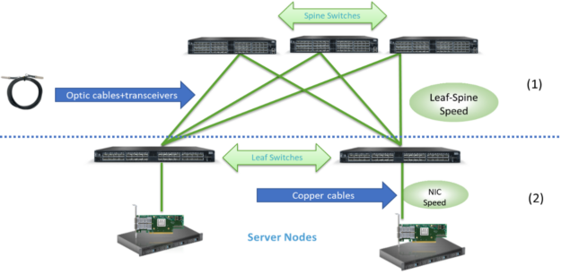

 Over the past couple of years, NVIDIA and NASA have been working closely on accelerating data science workflows using RAPIDS and integrating these GPU-accelerated libraries with scientific use cases. In this blog, we’ll share some of the results from an atmospheric science use case, and code snippets to port existing CPU workflows to RAPIDS on …

 With everyone shifting to a remote work environment, game development and professional visualization teams around the world need a solution for real-time collaboration and more efficient workflows.