
Six companies with innovative products built using the NVIDIA Jetson edge AI platform will leave CES, one of the world’s largest consumer technology trade shows, as big winners next week. The CES Innovation Awards each year honor outstanding design and engineering in more than two dozen categories of consumer technology products. The companies to be Read article >
These explainers will give you the scoop on the latest tech developments from AI models to green computing.
Artist Zhelong Xu, aka Uncle Light, brought to life Blood Moon — a 3D masterpiece combining imagination, craftsmanship and art styles from the Chinese Bronze Age — along with Kirin, a symbol of hope and good fortune, using NVIDIA technologies.

Major recent advances in multiple subfields of machine learning (ML) research, such as computer vision and natural language processing, have been enabled by a shared common approach that leverages large, diverse datasets and expressive models that can absorb all of the data effectively. Although there have been various attempts to apply this approach to robotics, robots have not yet leveraged highly-capable models as well as other subfields.
Several factors contribute to this challenge. First, there’s the lack of large-scale and diverse robotic data, which limits a model’s ability to absorb a broad set of robotic experiences. Data collection is particularly expensive and challenging for robotics because dataset curation requires engineering-heavy autonomous operation, or demonstrations collected using human teleoperations. A second factor is the lack of expressive, scalable, and fast-enough-for-real-time-inference models that can learn from such datasets and generalize effectively.
To address these challenges, we propose the Robotics Transformer 1 (RT-1), a multi-task model that tokenizes robot inputs and outputs actions (e.g., camera images, task instructions, and motor commands) to enable efficient inference at runtime, which makes real-time control feasible. This model is trained on a large-scale, real-world robotics dataset of 130k episodes that cover 700+ tasks, collected using a fleet of 13 robots from Everyday Robots (EDR) over 17 months. We demonstrate that RT-1 can exhibit significantly improved zero-shot generalization to new tasks, environments and objects compared to prior techniques. Moreover, we carefully evaluate and ablate many of the design choices in the model and training set, analyzing the effects of tokenization, action representation, and dataset composition. Finally, we’re open-sourcing the RT-1 code, and hope it will provide a valuable resource for future research on scaling up robot learning.
 |
| RT-1 absorbs large amounts of data, including robot trajectories with multiple tasks, objects and environments, resulting in better performance and generalization. |
Robotics Transformer (RT-1)
RT-1 is built on a transformer architecture that takes a short history of images from a robot’s camera along with task descriptions expressed in natural language as inputs and directly outputs tokenized actions.
RT-1’s architecture is similar to that of a contemporary decoder-only sequence model trained against a standard categorical cross-entropy objective with causal masking. Its key features include: image tokenization, action tokenization, and token compression, described below.
Image tokenization: We pass images through an EfficientNet-B3 model that is pre-trained on ImageNet, and then flatten the resulting 9×9×512 spatial feature map to 81 tokens. The image tokenizer is conditioned on natural language task instructions, and uses FiLM layers initialized to identity to extract task-relevant image features early on.
Action tokenization: The robot’s action dimensions are 7 variables for arm movement (x, y, z, roll, pitch, yaw, gripper opening), 3 variables for base movement (x, y, yaw), and an extra discrete variable to switch between three modes: controlling arm, controlling base, or terminating the episode. Each action dimension is discretized into 256 bins.
Token Compression: The model adaptively selects soft combinations of image tokens that can be compressed based on their impact towards learning with the element-wise attention module TokenLearner, resulting in over 2.4x inference speed-up.
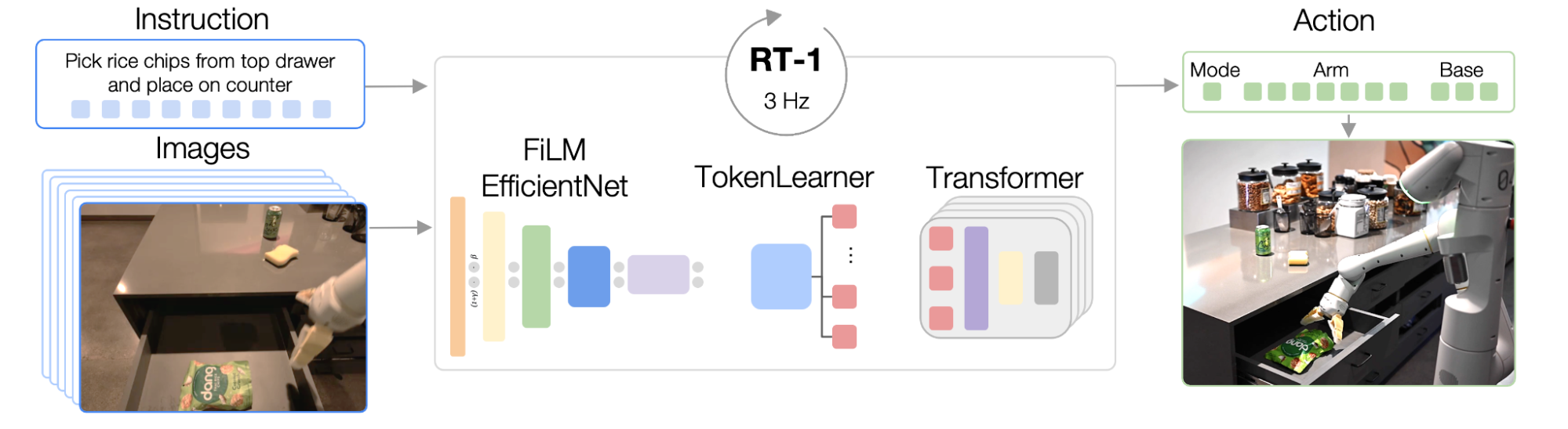 |
| RT-1’s architecture: The model takes a text instruction and set of images as inputs, encodes them as tokens via a pre-trained FiLM EfficientNet model and compresses them via TokenLearner. These are then fed into the Transformer, which outputs action tokens. |
To build a system that could generalize to new tasks and show robustness to different distractors and backgrounds, we collected a large, diverse dataset of robot trajectories. We used 13 EDR robot manipulators, each with a 7-degree-of-freedom arm, a 2-fingered gripper, and a mobile base, to collect 130k episodes over 17 months. We used demonstrations provided by humans through remote teleoperation, and annotated each episode with a textual description of the instruction that the robot just performed. The set of high-level skills represented in the dataset includes picking and placing items, opening and closing drawers, getting items in and out drawers, placing elongated items up-right, knocking objects over, pulling napkins and opening jars. The resulting dataset includes 130k+ episodes that cover 700+ tasks using many different objects.
Experiments and Results
To better understand RT-1’s generalization abilities, we study its performance against three baselines: Gato, BC-Z and BC-Z XL (i.e., BC-Z with same number of parameters as RT-1), across four categories:
- Seen tasks performance: performance on tasks seen during training
- Unseen tasks performance: performance on unseen tasks where the skill and object(s) were seen separately in the training set, but combined in novel ways
- Robustness (distractors and backgrounds): performance with distractors (up to 9 distractors and occlusion) and performance with background changes (new kitchen, lighting, background scenes)
- Long-horizon scenarios: execution of SayCan-type natural language instructions in a real kitchen
RT-1 outperforms baselines by large margins in all four categories, exhibiting impressive degrees of generalization and robustness.
 |
| Performance of RT-1 vs. baselines on evaluation scenarios. |
Incorporating Heterogeneous Data Sources
To push RT-1 further, we train it on data gathered from another robot to test if (1) the model retains its performance on the original tasks when a new data source is presented and (2) if the model sees a boost in generalization with new and different data, both of which are desirable for a general robot learning model. Specifically, we use 209k episodes of indiscriminate grasping that were autonomously collected on a fixed-base Kuka arm for the QT-Opt project. We transform the data collected to match the action specs and bounds of our original dataset collected with EDR, and label every episode with the task instruction “pick anything” (the Kuka dataset doesn’t have object labels). Kuka data is then mixed with EDR data in a 1:2 ratio in every training batch to control for regression in original EDR skills.
 |
| Training methodology when data has been collected from multiple robots. |
Our results indicate that RT-1 is able to acquire new skills by observing other robots’ experiences. In particular, the 22% accuracy seen when training with EDR data alone jumps by almost 2x to 39% when RT-1 is trained on both bin-picking data from Kuka and existing EDR data from robot classrooms, where we collected most of RT-1 data. When training RT-1 on bin-picking data from Kuka alone, and then evaluating it on bin-picking from the EDR robot, we see 0% accuracy. Mixing data from both robots, on the other hand, allows RT-1 to infer the actions of the EDR robot when faced with the states observed by Kuka, without explicit demonstrations of bin-picking on the EDR robot, and by taking advantage of experiences collected by Kuka. This presents an opportunity for future work to combine more multi-robot datasets to enhance robot capabilities.
| Training Data | Classroom Eval | Bin-picking Eval |
| Kuka bin-picking data + EDR data | 90% | 39% |
| EDR only data | 92% | 22% |
| Kuka bin-picking only data | 0 | 0 |
| RT-1 accuracy evaluation using various training data. |
Long-Horizon SayCan Tasks
RT-1’s high performance and generalization abilities can enable long-horizon, mobile manipulation tasks through SayCan. SayCan works by grounding language models in robotic affordances, and leveraging few-shot prompting to break down a long-horizon task expressed in natural language into a sequence of low-level skills.
SayCan tasks present an ideal evaluation setting to test various features:
- Long-horizon task success falls exponentially with task length, so high manipulation success is important.
- Mobile manipulation tasks require multiple handoffs between navigation and manipulation, so the robustness to variations in initial policy conditions (e.g., base position) is essential.
- The number of possible high-level instructions increases combinatorially with skill-breadth of the manipulation primitive.
We evaluate SayCan with RT-1 and two other baselines (SayCan with Gato and SayCan with BC-Z) in two real kitchens. Below, “Kitchen2” constitutes a much more challenging generalization scene than “Kitchen1”. The mock kitchen used to gather most of the training data was modeled after Kitchen1.
SayCan with RT-1 achieves a 67% execution success rate in Kitchen1, outperforming other baselines. Due to the generalization difficulty presented by the new unseen kitchen, the performance of SayCan with Gato and SayCan with BCZ shapely falls, while RT-1 does not show a visible drop.
| SayCan tasks in Kitchen1 | SayCan tasks in Kitchen2 | |||
| Planning | Execution | Planning | Execution | |
| Original Saycan | 73 | 47 | – | – |
| SayCan w/ Gato | 87 | 33 | 87 | 0 |
| SayCan w/ BC-Z | 87 | 53 | 87 | 13 |
| SayCan w/ RT-1 | 87 | 67 | 87 | 67 |
The following video shows a few example PaLM-SayCan-RT1 executions of long-horizon tasks in multiple real kitchens.
Conclusion
The RT-1 Robotics Transformer is a simple and scalable action-generation model for real-world robotics tasks. It tokenizes all inputs and outputs, and uses a pre-trained EfficientNet model with early language fusion, and a token learner for compression. RT-1 shows strong performance across hundreds of tasks, and extensive generalization abilities and robustness in real-world settings.
As we explore future directions for this work, we hope to scale the number of robot skills faster by developing methods that allow non-experts to train the robot with directed data collection and model prompting. We also look forward to improving robotics transformers’ reaction speeds and context retention with scalable attention and memory. To learn more, check out the paper, open-sourced RT-1 code, and the project website.
Acknowledgements
This work was done in collaboration with Anthony Brohan, Noah Brown, Justice Carbajal, Yevgen Chebotar, Joseph Dabis, Chelsea Finn, Keerthana Gopalakrishnan, Karol Hausman, Alex Herzog, Jasmine Hsu, Julian Ibarz, Brian Ichter, Alex Irpan, Tomas Jackson, Sally Jesmonth, Nikhil Joshi, Ryan Julian, Dmitry Kalashnikov, Yuheng Kuang, Isabel Leal, Kuang-Huei Lee, Sergey Levine, Yao Lu, Utsav Malla, Deeksha Manjunath, Igor Mordatch, Ofir Nachum, Carolina Parada, Jodilyn Peralta, Emily Perez, Karl Pertsch, Jornell Quiambao, Kanishka Rao, Michael Ryoo, Grecia Salazar, Pannag Sanketi, Kevin Sayed, Jaspiar Singh, Sumedh Sontakke, Austin Stone, Clayton Tan, Huong Tran, Vincent Vanhoucke, Steve Vega, Quan Vuong, Fei Xia, Ted Xiao, Peng Xu, Sichun Xu, Tianhe Yu, and Brianna Zitkovich.
In 2019 we launched Recorder, an audio recording app for Pixel phones that helps users create, manage, and edit audio recordings. It leverages recent developments in on-device machine learning to transcribe speech, recognize audio events, suggest tags for titles, and help users navigate transcripts.
Nonetheless, some Recorder users found it difficult to navigate long recordings that have multiple speakers because it’s not clear who said what. During the Made By Google event this year, we announced the “speaker labels” feature for the Recorder app. This opt-in feature annotates a recording transcript with unique and anonymous labels for each speaker (e.g., “Speaker 1”, “Speaker 2”, etc.) in real time during the recording. It significantly improves the readability and usability of the recording transcripts. This feature is powered by Google’s new speaker diarization system named Turn-to-Diarize, which was first presented at ICASSP 2022.
|
| Left: Recorder transcript without speaker labels. Right: Recorder transcript with speaker labels. |
System Architecture
Our speaker diarization system leverages several highly optimized machine learning models and algorithms to allow diarizing hours of audio in a real-time streaming fashion with limited computational resources on mobile devices. The system mainly consists of three components: a speaker turn detection model that detects a change of speaker in the input speech, a speaker encoder model that extracts voice characteristics from each speaker turn, and a multi-stage clustering algorithm that annotates speaker labels to each speaker turn in a highly efficient way. All components run fully on the device.
 |
| Architecture of the Turn-to-Diarize system. |
Detecting Speaker Turns
The first component of our system is a speaker turn detection model based on a Transformer Transducer (T-T), which converts the acoustic features into text transcripts augmented with a special token <st> representing a speaker turn. Unlike preceding customized systems that use role-specific tokens (e.g., <doctor> and <patient>) for conversations, this model is more generic and can be trained on and deployed to various application domains.
In most applications, the output of a diarization system is not directly shown to users, but combined with a separate automatic speech recognition (ASR) system that is trained to have smaller word errors. Therefore, for the diarization system, we are relatively more tolerant to word token errors than errors of the <st> token. Based on this intuition, we propose a new token-level loss function that allows us to train a small speaker turn detection model with high accuracy on predicted <st> tokens. Combined with edit-based minimum Bayes risk (EMBR) training, this new loss function significantly improved the interval-based F1 score on seven evaluation datasets.
Extracting Voice Characteristics
Once the audio recording has been segmented into homogeneous speaker turns, we use a speaker encoder model to extract an embedding vector (i.e., d-vector) to represent the voice characteristics of each speaker turn. This approach has several advantages over prior work that extracts embedding vectors from small fixed-length segments. First, it avoids extracting an embedding from a segment containing speech from multiple speakers. At the same time, each embedding covers a relatively large time range that contains sufficient signals from the speaker. It also reduces the total number of embeddings to be clustered, thus making the clustering step less expensive. These embeddings are processed entirely on-device until speaker labeling of the transcript is completed, and then deleted.
Multi-Stage Clustering
After the audio recording is represented by a sequence of embedding vectors, the last step is to cluster these embedding vectors, and assign a speaker label to each. However, since audio recordings from the Recorder app can be as short as a few seconds, or as long as up to 18 hours, it is critical for the clustering algorithm to handle sequences of drastically different lengths.
For this we propose a multi-stage clustering strategy to leverage the benefits of different clustering algorithms. First, we use the speaker turn detection outputs to determine whether there are at least two different speakers in the recording. For short sequences, we use agglomerative hierarchical clustering (AHC) as the fallback algorithm. For medium-length sequences, we use spectral clustering as our main algorithm, and use the eigen-gap criterion for accurate speaker count estimation. For long sequences, we reduce computational cost by using AHC to pre-cluster the sequence before feeding it to the main algorithm. During the streaming, we keep a dynamic cache of previous AHC cluster centroids that can be reused for future clustering calls. This mechanism allows us to enforce an upper bound on the entire system with constant time and space complexity.
This multi-stage clustering strategy is a critical optimization for on-device applications where the budget for CPU, memory, and battery is very small, and allows the system to run in a low power mode even after diarizing hours of audio. As a tradeoff between quality and efficiency, the upper bound of the computational cost can be flexibly configured for devices with different computational resources.
 |
| Diagram of the multi-stage clustering strategy. |
Correction and Customization
In our real-time streaming speaker diarization system, as the model consumes more audio input, it accumulates confidence on predicted speaker labels, and may occasionally make corrections to previously predicted low-confidence speaker labels. The Recorder app automatically updates the speaker labels on the screen during recording to reflect the latest and most accurate predictions.
At the same time, the Recorder app’s UI allows the user to rename the anonymous speaker labels (e.g., “Speaker 2”) to customized labels (e.g., “car dealer”) for better readability and easier memorization for the user within each recording.
 |
| Recorder allows the user to rename the speaker labels for better readability. |
Future Work
Currently, our diarization system mostly runs on the CPU block of Google Tensor, Google’s custom-built chip that powers more recent Pixel phones. We are working on delegating more computations to the TPU block, which will further reduce the overall power consumption of the diarization system. Another future work direction is to leverage multilingual capabilities of speaker encoder and speech recognition models to expand this feature to more languages.
Acknowledgments
The work described in this post represents joint efforts from multiple teams within Google. Contributors include Quan Wang, Yiling Huang, Evan Clark, Qi Cao, Han Lu, Guanlong Zhao, Wei Xia, Hasim Sak, Alvin Zhou, Jason Pelecanos, Luiza Timariu, Allen Su, Fan Zhang, Hugh Love, Kristi Bradford, Vincent Peng, Raff Tsai, Richard Chou, Yitong Lin, Ann Lu, Kelly Tsai, Hannah Bowman, Tracy Wu, Taral Joglekar, Dharmesh Mokani, Ajay Dudani, Ignacio Lopez Moreno, Diego Melendo Casado, Nino Tasca, Alex Gruenstein.
Language models (LMs) are the driving force behind many recent breakthroughs in natural language processing. Models like T5, LaMDA, GPT-3, and PaLM have demonstrated impressive performance on various language tasks. While multiple factors can contribute to improving the performance of LMs, some recent studies suggest that scaling up the model’s size is crucial for revealing emergent capabilities. In other words, some instances can be solved by small models, while others seem to benefit from increased scale.
Despite recent efforts that enabled the efficient training of LMs over large amounts of data, trained models can still be slow and costly for practical use. When generating text at inference time, most autoregressive LMs output content similar to how we speak and write (word after word), predicting each new word based on the preceding words. This process cannot be parallelized since LMs need to complete the prediction of one word before starting to compute the next one. Moreover, predicting each word requires significant computation given the model’s billions of parameters.
In “Confident Adaptive Language Modeling”, presented at NeurIPS 2022, we introduce a new method for accelerating the text generation of LMs by improving efficiency at inference time. Our method, named CALM, is motivated by the intuition that some next word predictions are easier than others. When writing a sentence, some continuations are trivial, while others might require more effort. Current LMs devote the same amount of compute power for all predictions. Instead, CALM dynamically distributes the computational effort across generation timesteps. By selectively allocating more computational resources only to harder predictions, CALM generates text faster while preserving output quality.
Confident Adaptive Language Modeling
When possible, CALM skips some compute effort for certain predictions. To demonstrate this, we use the popular encoder-decoder T5 architecture. The encoder reads the input text (e.g., a news article to summarize) and converts the text to dense representations. Then, the decoder outputs the summary by predicting it word by word. Both the encoder and decoder include a long sequence of Transformer layers. Each layer includes attention and feedforward modules with many matrix multiplications. These layers gradually modify the hidden representation that is ultimately used for predicting the next word.
Instead of waiting for all decoder layers to complete, CALM attempts to predict the next word earlier, after some intermediate layer. To decide whether to commit to a certain prediction or to postpone the prediction to a later layer, we measure the model’s confidence in its intermediate prediction. The rest of the computation is skipped only when the model is confident enough that the prediction won’t change. For quantifying what is “confident enough”, we calibrate a threshold that statistically satisfies arbitrary quality guarantees over the full output sequence.
 |
| Text generation with a regular language model (top) and with CALM (bottom). CALM attempts to make early predictions. Once confident enough (darker blue tones), it skips ahead and saves time. |
Language Models with Early Exits
Enabling this early exit strategy for LMs requires minimal modifications to the training and inference processes. During training, we encourage the model to produce meaningful representations in intermediate layers. Instead of predicting only using the top layer, our learning loss function is a weighted average over the predictions of all layers, assigning higher weight to top layers. Our experiments demonstrate that this significantly improves the intermediate layer predictions while preserving the full model’s performance. In one model variant, we also include a small early-exit classifier trained to classify if the local intermediate layer prediction is consistent with the top layer. We train this classifier in a second quick step where we freeze the rest of the model.
Once the model is trained, we need a method to allow early-exiting. First, we define a local confidence measure for capturing the model’s confidence in its intermediate prediction. We explore three confidence measures (described in the results section below): (1) softmax response, taking the maximum predicted probability out of the softmax distribution; (2) state propagation, the cosine distance between the current hidden representation and the one from the previous layer; and (3) early-exit classifier, the output of a classifier specifically trained for predicting local consistency. We find the softmax response to be statistically strong while being simple and fast to compute. The other two alternatives are lighter in floating point operations (FLOPS).
Another challenge is that the self-attention of each layer depends on hidden-states from previous words. If we exit early for some word predictions, these hidden-states might be missing. Instead, we attend back to the hidden state of the last computed layer.
Finally, we set up the local confidence threshold for exiting early. In the next section, we describe our controlled process for finding good threshold values. As a first step, we simplify this infinite search space by building on a useful observation: mistakes that are made at the beginning of the generation process are more detrimental since they can affect all of the following outputs. Therefore, we start with a higher (more conservative) threshold, and gradually reduce it with time. We use a negative exponent with user-defined temperature to control this decay rate. We find this allows better control over the performance-efficiency tradeoff (the obtained speedup per quality level).
Reliably Controlling the Quality of the Accelerated Model
Early exit decisions have to be local; they need to happen when predicting each word. In practice, however, the final output should be globally consistent or comparable to the original model. For example, if the original full model generated “the concert was wonderful and long”, one would accept CALM switching the order of the adjectives and outputting “the concert was long and wonderful”. However, at the local level, the word “wonderful” was replaced with “long”. Therefore, the two outputs are globally consistent, but include some local inconsistencies. We build on the Learn then Test (LTT) framework to connect local confidence-based decisions to globally consistent outputs.
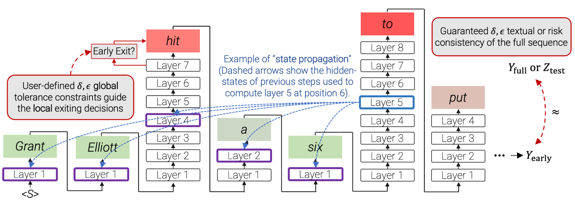 |
| In CALM, local per-timestep confidence thresholds for early exiting decisions are derived, via LTT calibration, from user-defined consistency constraints over the full output text. Red boxes indicate that CALM used most of the decoder’s layers for that specific prediction. Green boxes indicate that CALM saved time by using only a few Transformer layers. Full sentence shown in the last example of this post. |
First, we define and formulate two types of consistency constraints from which to choose:
- Textual consistency: We bound the expected textual distance between the outputs of CALM and the outputs of the full model. This doesn’t require any labeled data.
- Risk consistency: We bound the expected increase in loss that we allow for CALM compared to the full model. This requires reference outputs against which to compare.
For each of these constraints, we can set the tolerance that we allow and calibrate the confidence threshold to allow early exits while reliably satisfying our defined constraint with an arbitrarily high probability.
CALM Saves Inference Time
We run experiments on three popular generation datasets: CNN/DM for summarization, WMT for machine translation, and SQuAD for question answering. We evaluate each of the three confidence measures (softmax response, state propagation and early-exit classifier) using an 8-layer encoder-decoder model. To evaluate global sequence-level performance, we use the standard Rouge-L, BLEU, and Token-F1 scores that measure distances against human-written references. We show that one can maintain full model performance while using only a third or half of the layers on average. CALM achieves this by dynamically distributing the compute effort across the prediction timesteps.
As an approximate upper bound, we also compute the predictions using a local oracle confidence measure, which enables exiting at the first layer that leads to the same prediction as the top one. On all three tasks, the oracle measure can preserve full model performance when using only 1.5 decoder layers on average. In contrast to CALM, a static baseline uses the same number of layers for all predictions, requiring 3 to 7 layers (depending on the dataset) to preserve its performance. This demonstrates why the dynamic allocation of compute effort is important. Only a small fraction of the predictions require most of the model’s complexity, while for others much less should suffice.
 |
| Performance per task against the average number of decoder layers used. |
Finally, we also find that CALM enables practical speedups. When benchmarking on TPUs, we saved almost half of the compute time while maintaining the quality of the outputs.
 |
| Example of a generated news summary. The top cell presents the reference human-written summary. Below is the prediction of the full model (8 layers) followed by two different CALM output examples. The first CALM output is 2.9x faster and the second output is 3.6x faster than the full model, benchmarked on TPUs. |
Conclusion
CALM allows faster text generation with LMs, without reducing the quality of the output text. This is achieved by dynamically modifying the amount of compute per generation timestep, allowing the model to exit the computational sequence early when confident enough.
As language models continue to grow in size, studying how to efficiently use them becomes crucial. CALM is orthogonal and can be combined with many efficiency related efforts, including model quantization, distillation, sparsity, effective partitioning, and distributed control flows.
Acknowledgements
It was an honor and privilege to work on this with Adam Fisch, Ionel Gog, Seungyeon Kim, Jai Gupta, Mostafa Dehghani, Dara Bahri, Vinh Q. Tran, Yi Tay, and Donald Metzler. We also thank Anselm Levskaya, Hyung Won Chung, Tao Wang, Paul Barham, Michael Isard, Orhan Firat, Carlos Riquelme, Aditya Menon, Zhifeng Chen, Sanjiv Kumar, and Jeff Dean for helpful discussions and feedback. Finally, we thank Tom Small for preparing the animation in this blog post.
Differential privacy (DP) is an approach that enables data analytics and machine learning (ML) with a mathematical guarantee on the privacy of user data. DP quantifies the “privacy cost” of an algorithm, i.e., the level of guarantee that the algorithm’s output distribution for a given dataset will not change significantly if a single user’s data is added to or removed from it. The algorithm is characterized by two parameters, ε and δ, where smaller values of both indicate “more private”. There is a natural tension between the privacy budget (ε, δ) and the utility of the algorithm: a smaller privacy budget requires the output to be more “noisy”, often leading to less utility. Thus, a fundamental goal of DP is to attain as much utility as possible for a desired privacy budget.
A key property of DP that often plays a central role in understanding privacy costs is that of composition, which reflects the net privacy cost of a combination of DP algorithms, viewed together as a single algorithm. A notable example is the differentially-private stochastic gradient descent (DP-SGD) algorithm. This algorithm trains ML models over multiple iterations — each of which is differentially private — and therefore requires an application of the composition property of DP. A basic composition theorem in DP says that the privacy cost of a collection of algorithms is, at most, the sum of the privacy cost of each. However, in many cases, this can be a gross overestimate, and several improved composition theorems provide better estimates of the privacy cost of composition.
In 2019, we released an open-source library (on GitHub) to enable developers to use analytic techniques based on DP. Today, we announce the addition to this library of Connect-the-Dots, a new privacy accounting algorithm based on a novel approach for discretizing privacy loss distributions that is a useful tool for understanding the privacy cost of composition. This algorithm is based on the paper “Connect the Dots: Tighter Discrete Approximations of Privacy Loss Distributions”, presented at PETS 2022. The main novelty of this accounting algorithm is that it uses an indirect approach to construct more accurate discretizations of privacy loss distributions. We find that Connect-the-Dots provides significant gains over other privacy accounting methods in literature in terms of accuracy and running time. This algorithm was also recently applied for the privacy accounting of DP-SGD in training Ads prediction models.
Differential Privacy and Privacy Loss Distributions
A randomized algorithm is said to satisfy DP guarantees if its output “does not depend significantly” on any one entry in its training dataset, quantified mathematically with parameters (ε, δ). For example, consider the motivating example of DP-SGD. When trained with (non-private) SGD, a neural network could, in principle, be encoding the entire training dataset within its weights, thereby allowing one to reconstruct some training examples from a trained model. On the other hand, when trained with DP-SGD, we have a formal guarantee that if one were able to reconstruct a training example with non-trivial probability then one would also be able to reconstruct the same example even if it was not included in the training dataset.
The hockey stick divergence, parameterized by ε, is a measure of distance between two probability distributions, as illustrated in the figure below. The privacy cost of most DP algorithms is dictated by the hockey stick divergence between two associated probability distributions P and Q. The algorithm satisfies DP with parameters (ε, δ), if the value of the hockey stick divergence for ε between P and Q is at most δ. The hockey stick divergence between (P, Q), denoted δP||Q(ε) is in turn completely characterized by it associated privacy loss distribution, denoted by PLDP||Q.
 |
| Illustration of hockey stick divergence δP||Q(ε) between distributions P and Q (left), which corresponds to the probability mass of P that is above eεQ, where eεQ is an eε scaling of the probability mass of Q (right). |
The main advantage of dealing with PLDs is that compositions of algorithms correspond to the convolution of the corresponding PLDs. Exploiting this fact, prior work has designed efficient algorithms to compute the PLD corresponding to the composition of individual algorithms by simply performing convolution of the individual PLDs using the fast Fourier transform algorithm.
However, one challenge when dealing with many PLDs is that they often are continuous distributions, which make the convolution operations intractable in practice. Thus, researchers often apply various discretization approaches to approximate the PLDs using equally spaced points. For example, the basic version of the Privacy Buckets algorithm assigns the probability mass of the interval between two discretization points entirely to the higher end of the interval.
 |
| Illustration of discretization by rounding up probability masses. Here a continuous PLD (in blue) is discretized to a discrete PLD (in red), by rounding up the probability mass between consecutive points. |
Connect-the-Dots : A New Algorithm
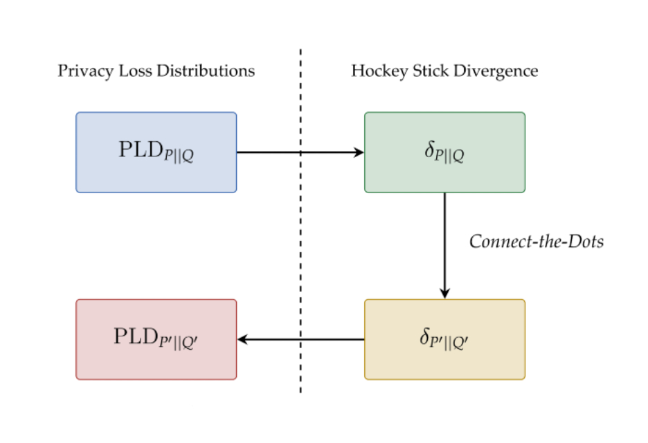
Our new Connect-the-Dots algorithm provides a better way to discretize PLDs towards the goal of estimating hockey stick divergences. This approach works indirectly by first discretizing the hockey stick divergence function and then mapping it back to a discrete PLD supported on equally spaced points.
 |
| Illustration of high-level steps in the Connect-the-Dots algorithm. |
This approach relies on the notion of a “dominating PLD”, namely, PLDP’||Q’ dominates over PLDP||Q if the hockey stick divergence of the former is greater or equal to the hockey stick divergence of the latter for all values of ε. The key property of dominating PLDs is that they remain dominating after compositions. Thus for purposes of privacy accounting, it suffices to work with a dominating PLD, which gives us an upper bound on the exact privacy cost.
Our main insight behind the Connect-the-Dots algorithm is a characterization of discrete PLD, namely that a PLD is supported on a given finite set of ε values if and only if the corresponding hockey stick divergence as a function of eε is linear between consecutive eε values. This allows us to discretize the hockey stick divergence by simply connecting the dots to get a piecewise linear function that precisely equals the hockey stick divergence function at the given eε values. See a more detailed explanation of the algorithm.
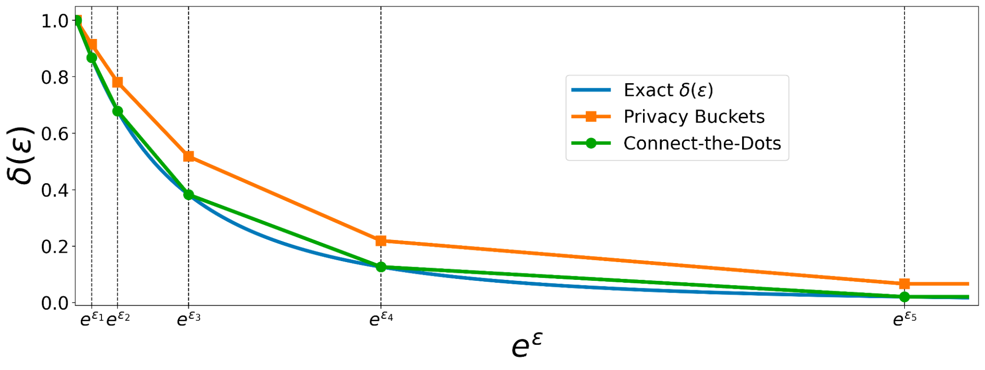 |
| Comparison of the discretizations of hockey stick divergence by Connect-the-Dots vs Privacy Buckets. |
Experimental Evaluation
The DP-SGD algorithm involves a noise multiplier parameter, which controls the magnitude of noise added in each gradient step, and a sampling probability, which controls how many examples are included in each mini-batch. We compare Connect-the-Dots against the algorithms listed below on the task of privacy accounting DP-SGD with a noise multiplier = 0.5, sampling probability = 0.2 x 10⁻⁴ and δ = 10-8.
- Renyi DP : The original approach used for the privacy accounting of DP-SGD. This accounting method is also supported in the Google-DP library.
- Privacy Buckets : The previous PLD-based approach used in Google-DP library, which rounds up probability masses between discretization points.
- Microsoft PRV Accountant : This approach improves upon the Privacy Buckets approach using a discretization that preserves the mean of the PLD.
We plot the value of the ε computed by each of the algorithms against the number of composition steps, and additionally, we plot the running time of the implementations. As shown in the plots below, privacy accounting using Renyi DP provides a loose estimate of the privacy loss. However, when comparing the approaches using PLD, we find that in this example, the implementation of Connect-the-Dots achieves a tighter estimate of the privacy loss, with a running time that is 5x faster than the Microsoft PRV Accountant and >200x faster than the previous approach of Privacy Buckets in the Google-DP library.
 |
| Left: Upper bounds on the privacy parameter ε for varying number of steps of DP-SGD, as returned by different algorithms (for fixed δ = 10-8). Right: Running time of the different algorithms. |
Conclusion & Future Directions
This work proposes Connect-the-Dots, a new algorithm for computing optimal privacy parameters for compositions of differentially private algorithms. When evaluated on the DP-SGD task, we find that this algorithm gives tighter estimates on the privacy loss with a significantly faster running time.
So far, the library only supports the pessimistic estimate version of Connect-the-Dots algorithm, which provides an upper bound on the privacy loss of DP-algorithms. However, the paper also introduces a variant of the algorithm that provides an “optimistic” estimate of the PLD, which can be used to derive lower bounds on the privacy cost of DP-algorithms (provided those admit a “worst case” PLD). Currently, the library does support optimistic estimates as given by the Privacy Buckets algorithm, and we hope to incorporate the Connect-the-Dots version as well.
Acknowledgements
This work was carried out in collaboration with Vadym Doroshenko, Badih Ghazi, Ravi Kumar. We thank Galen Andrew, Stan Bashtavenko, Steve Chien, Christoph Dibak, Miguel Guevara, Peter Kairouz, Sasha Kulankhina, Stefan Mellem, Jodi Spacek, Yurii Sushko and Andreas Terzis for their help.

Analysis of Electronic Health Records (EHR) has a tremendous potential for enhancing patient care, quantitatively measuring performance of clinical practices, and facilitating clinical research. Statistical estimation and machine learning (ML) models trained on EHR data can be used to predict the probability of various diseases (such as diabetes), track patient wellness, and predict how patients respond to specific drugs. For such models, researchers and practitioners need access to EHR data. However, it can be challenging to leverage EHR data while ensuring data privacy and conforming to patient confidentiality regulations (such as HIPAA).
Conventional methods to anonymize data (e.g., de-identification) are often tedious and costly. Moreover, they can distort important features from the original dataset, decreasing the utility of the data significantly; they can also be susceptible to privacy attacks. Alternatively, an approach based on generating synthetic data can maintain both important dataset features and privacy.
To that end, we propose a novel generative modeling framework in “EHR-Safe: Generating High-Fidelity and Privacy-Preserving Synthetic Electronic Health Records“. With the innovative methodology in EHR-Safe, we show that synthetic data can satisfy two key properties: (i) high fidelity (i.e., they are useful for the task of interest, such as having similar downstream performance when a diagnostic model is trained on them), (ii) meet certain privacy measures (i.e., they do not reveal any real patient’s identity). Our state-of-the-art results stem from novel approaches for encoding/decoding features, normalizing complex distributions, conditioning adversarial training, and representing missing data.
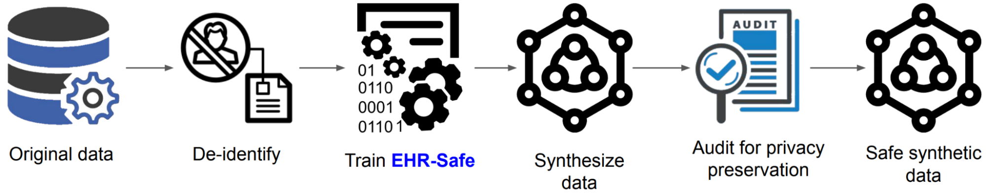 |
| Generating synthetic data from the original data with EHR-Safe. |
Challenges of Generating Realistic Synthetic EHR Data
There are multiple fundamental challenges to generating synthetic EHR data. EHR data contain heterogeneous features with different characteristics and distributions. There can be numerical features (e.g., blood pressure) and categorical features with many or two categories (e.g., medical codes, mortality outcome). Some of these may be static (i.e., not varying during the modeling window), while others are time-varying, such as regular or sporadic lab measurements. Distributions might come from different families — categorical distributions can be highly non-uniform (e.g., for under-represented groups) and numerical distributions can be highly skewed (e.g., a small proportion of values being very large while the vast majority are small). Depending on a patient’s condition, the number of visits can also vary drastically — some patients visit a clinic only once whereas some visit hundreds of times, leading to a variance in sequence lengths that is typically much higher compared to other time-series data. There can be a high ratio of missing features across different patients and time steps, as not all lab measurements or other input data are collected.
 |
 |
| Examples of real EHR data: temporal numerical features (upper) and temporal categorical features (lower). |
EHR-Safe: Synthetic EHR Data Generation Framework
EHR-Safe consists of sequential encoder-decoder architecture and generative adversarial networks (GANs), depicted in the figure below. Because EHR data are heterogeneous (as described above), direct modeling of raw EHR data is challenging for GANs. To circumvent this, we propose utilizing a sequential encoder-decoder architecture, to learn the mapping from the raw EHR data to the latent representations, and vice versa.
 |
| Block diagram of EHR-Safe framework. |
While learning the mapping, esoteric distributions of numerical and categorical features pose a great challenge. For example, some values or numerical ranges might dominate the distribution, but the capability of modeling rare cases is essential. The proposed feature mapping and stochastic normalization (transforming original feature distributions into uniform distributions without information loss) are key to handling such data by converting to distributions for which the training of encoder-decoder and GAN are more stable (details can be found in the paper). The mapped latent representations, generated by the encoder, are then used for GAN training. After training both the encoder-decoder framework and GANs, EHR-Safe can generate synthetic heterogeneous EHR data from any input, for which we feed randomly sampled vectors. Note that only the trained generator and decoders are used for generating synthetic data.
Datasets
We focus on two real-world EHR datasets to showcase the EHR-Safe framework, MIMIC-III and eICU. Both are inpatient datasets that consist of varying lengths of sequences and include multiple numerical and categorical features with missing components.
Fidelity Results
The fidelity metrics focus on the quality of synthetically generated data by measuring the realisticness of the synthetic data. Higher fidelity implies that it is more difficult to differentiate between synthetic and real data. We evaluate the fidelity of synthetic data in terms of multiple quantitative and qualitative analyses.
Visualization
Having similar coverage and avoiding under-representation of certain data regimes are both important for synthetic data generation. As the below t-SNE analyses show, the coverage of the synthetic data (blue) is very similar with the original data (red). With membership inference metrics (will be introduced in the privacy section), we also verify that EHR-Safe does not just memorize the original train data.
 |
| t-SNE analyses on temporal and static data on MIMIC-III (upper) and eICU (lower) datasets. |
Statistical Similarity
We provide quantitative comparisons of statistical similarity between original and synthetic data for each feature. Most statistics are well-aligned between original and synthetic data — for example a measure of the KS statistics, i.e,. the maximum difference in the cumulative distribution function (CDF) between the original and the synthetic data, are mostly lower than 0.03. More detailed tables can be found in the paper. The figure below exemplifies the CDF graphs for original vs. synthetic data for three features — overall they seem very close in most cases.
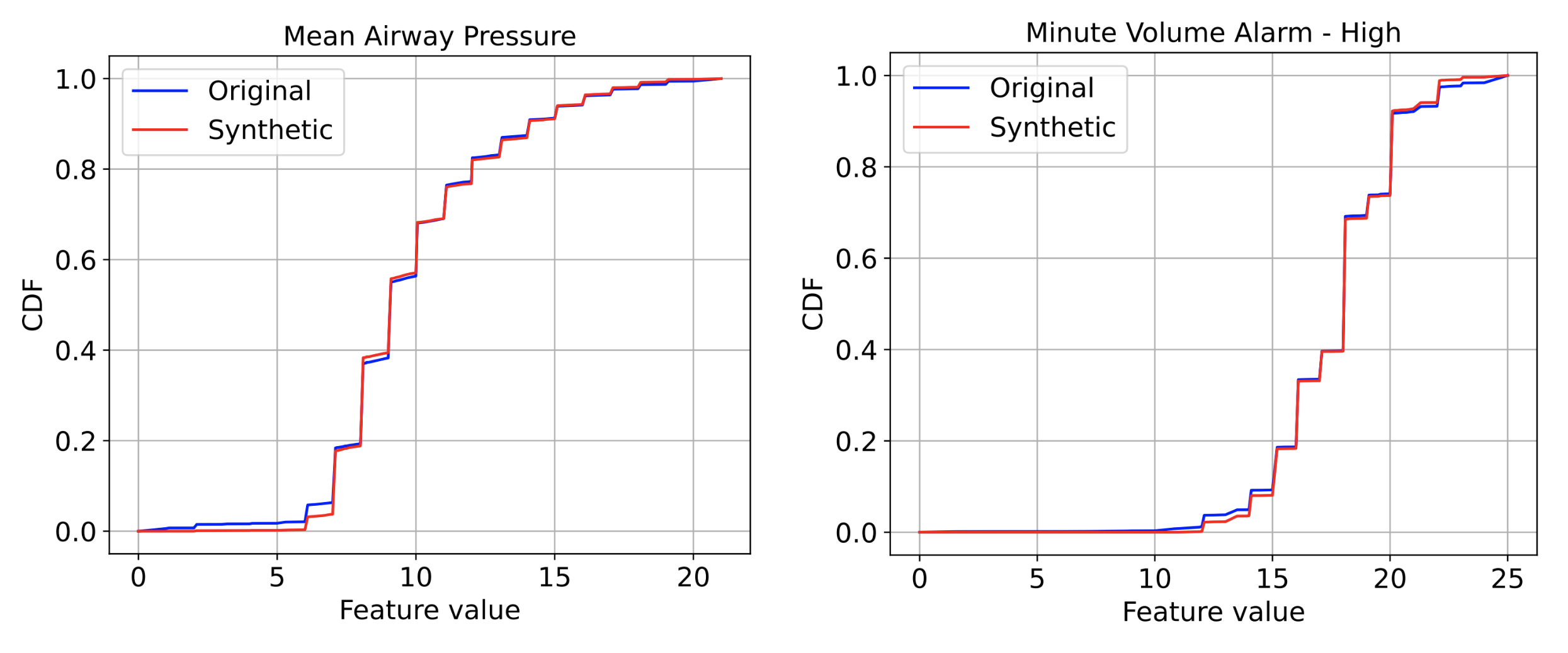 |
| CDF graphs of two features between original and synthetic EHR data. Left: Mean Airway Pressure. Right: Minute Volume Alarm. |
Utility
Because one of the most important use cases of synthetic data is enabling ML innovations, we focus on the fidelity metric that measures the ability of models trained on synthetic data to make accurate predictions on real data. We compare such model performance to an equivalent model trained with real data. Similar model performance would indicate that the synthetic data captures the relevant informative content for the task. As one of the important potential use cases of EHR, we focus on the mortality prediction task. We consider four different predictive models: Gradient Boosting Tree Ensemble (GBDT), Random Forest (RF), Logistic Regression (LR), Gated Recurrent Units (GRU).
 |
| Mortality prediction performance with the model trained on real vs. synthetic data. Left: MIMIC-III. Right: eICU. |
In the figure above we see that in most scenarios, training on synthetic vs. real data are highly similar in terms of Area Under Receiver Operating Characteristics Curve (AUC). On MIMIC-III, the best model (GBDT) on synthetic data is only 2.6% worse than the best model on real data; whereas on eICU, the best model (RF) on synthetic data is only 0.9% worse.
Privacy Results
We consider three different privacy attacks to quantify the robustness of the synthetic data with respect to privacy.
- Membership inference attack: An adversary predicts whether a known subject was a present in the training data used for training the synthetic data model.
- Re-identification attack: The adversary explores the probability of some features being re-identified using synthetic data and matching to the training data.
- Attribute inference attack: The adversary predicts the value of sensitive features using synthetic data.
 |
| Privacy risk evaluation across three privacy metrics: membership-inference (top-left), re-identification (top-right), and attribute inference (bottom). The ideal value of privacy risk for membership inference is random guessing (0.5). For re-identification, the ideal case is to replace the synthetic data with disjoint holdout original data. |
The figure above summarizes the results along with the ideal achievable value for each metric. We observe that the privacy metrics are very close to the ideal in all cases. The risk of understanding whether a sample of the original data is a member used for training the model is very close to random guessing; it also verifies that EHR-Safe does not just memorize the original train data. For the attribute inference attack, we focus on the prediction task of inferring specific attributes (e.g., gender, religion, and marital status) from other attributes. We compare prediction accuracy when training a classifier with real data against the same classifier trained with synthetic data. Because the EHR-Safe bars are all lower, the results demonstrate that access to synthetic data does not lead to higher prediction performance on specific features as compared to access to the original data.
Comparison to Alternative Methods
We compare EHR-Safe to alternatives (TimeGAN, RC-GAN, C-RNN-GAN) proposed for time-series synthetic data generation. As shown below, EHR-Safe significantly outperforms each.
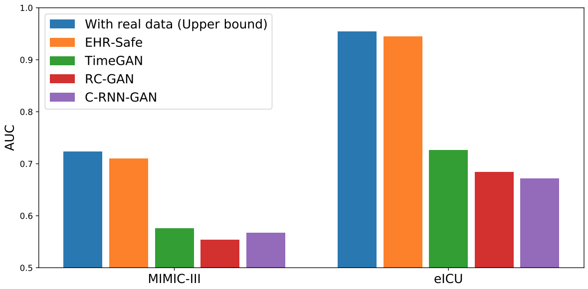 |
| Downstream task performance (AUC) in comparison to alternatives. |
Conclusions
We propose a novel generative modeling framework, EHR-Safe, that can generate highly realistic synthetic EHR data that are robust to privacy attacks. EHR-Safe is based on generative adversarial networks applied to the encoded raw data. We introduce multiple innovations in the architecture and training mechanisms that are motivated by the key challenges of EHR data. These innovations are key to our results that show almost-identical properties with real data (when desired downstream capabilities are considered) with almost-ideal privacy preservation. An important future direction is generative modeling capability for multimodal data, including text and image, as modern EHR data might contain both.
Acknowledgements
We gratefully acknowledge the contributions of Michel Mizrahi, Nahid Farhady Ghalaty, Thomas Jarvinen, Ashwin S. Ravi, Peter Brune, Fanyu Kong, Dave Anderson, George Lee, Arie Meir, Farhana Bandukwala, Elli Kanal, and Tomas Pfister.
In a moment of pure serendipity, Lah Yileh Lee and Xinting Lee, a pair of talented singers who often stream their performances online, found themselves performing in a public square in Taipei when NVIDIA founder and CEO Jensen Huang happened upon them. Huang couldn’t resist joining in, cheering on their serenade as they recorded Lady Read article >
The post Toy Jensen Rings in Holidays With AI-Powered ‘Jingle Bells’ appeared first on NVIDIA Blog.
This holiday season, feast on the bounty of food-themed stories NVIDIA Blog readers gobbled up in 2022. Startups in the retail industry — and particularly in quick-service restaurants — are using NVIDIA AI and robotics technology to make it easier to order food in drive-thrus, find beverages on store shelves and have meals delivered. They’re Read article >
The post Top Food Stories From 2022: Meet 4 Startups Putting AI on the Plate appeared first on NVIDIA Blog.