Categories
Misc

Tool for Complex Data Labelling Tasks

Hi /r/tensorflow
readers!

We have created a labelling
tool
that can be customized to display all sorts of data models
and tasks. Here are a couple of examples for NLP
and CV.

I hope some of you will find this useful, and if you have any
thoughts I would love to hear your feedback!

submitted by /u/bernatfp

[visit reddit]

[comments]

Categories
Misc

Constrain outputs in a regression problem

Hi, everyone.

I am attempting to constrain some outputs of my regression
network, say x, y, z = model(data), where x, y, z are scalars. The
constrain that I want to impose is that when predicting all three
dependent variables, the condition “x + y <=1.0” must be
honored. Given this description, can I implement this in a forward
function?

Thank you!

submitted by /u/ncuxomun

[visit reddit]

[comments]

Categories
Misc

Jetson Project of the Month: Blinkr – Blink Detection and Reminder

The project, which runs on a NVIDIA Jetson Nano 2GB Developer Kit, monitors the eyes of the user and voices a prompt when their blink rate is less than the recommended rate of 10 blinks per minute.

Thirteen-year-old Adrit Rao, was awarded the Jetson Project of the Month for his Blink Detection and Reminder (Blinkr). The project, which runs on a NVIDIA Jetson Nano 2GB Developer Kit, monitors the eyes of the user and voices a prompt when their blink rate is less than the recommended rate of 10 blinks per minute. 

Several studies have shown that low eye blinking rate, usually triggered by the use of a computer screen, is the leading cause of computer vision syndrome and other related disorders. To address this problem, Adrit created Blinkr with a simple setup of Jetson Nano 2GB Developer Kit, a webcam (or a Raspberry Pi v2 camera), a speaker and a few other basic peripherals.

The camera monitors the face of the user and feeds the frames to the Jetson Nano. To detect blinking, Adrit uses a 68 point facial landmark pre-trained model available in the Dlib open source library. Eyes are detected in each frame and the eye aspect ratio (EAR) is calculated and used to record the number of blinks over time. When the total blinks in a minute is less than the recommended rate, the speaker voices an alarm urging the user to blink more. 


Blinkr – Introduction video 

Many of us working from home do not have the usual prompts or interruptions during our day to move away from our screens. Tools like Blinkr can help us adopt healthy screen habits. This is a great project to build at home to learn about Jetson and AI, and to protect your eyesight. 

This project earned Adrit his Jetson AI Specialist certificate. We are keeping our appreciative (and healthy) eyes peeled out to see what he builds next. If you’re interested in building your own Blinkr, he has shared the instructions and the code here.

Categories
Misc

Dive into the Future of Graphics with NVIDIA Omniverse On-Demand Sessions

NVIDIA Omniverse is bringing the new standard in real-time graphics for developers. Check out some of the resources on the NVIDIA On-Demand catalog to learn more tips and tricks for developing in Omniverse.

NVIDIA Omniverse is bringing the new standard in real-time graphics for developers. Teams across industries are now using the open, cloud-native platform to deliver new levels of virtual collaboration and photorealistic simulation to their projects. And with open beta availability recently announced, more developers around the world can experience Omniverse and explore ways to integrate technologies or connect applications. 

Check out some of the resources on the NVIDIA On-Demand catalog to learn more tips and tricks for developing in Omniverse:

Getting Started with Omniverse Launcher: Learn more about the Omniverse Launcher as this session covers installation and configuration, as well as an overview of how to install applications and connectors. 

Omniverse Create Overview: Learn how Omniverse Create accelerates advanced scene composition and allows users to assemble, light, simulate, and render complex USD scenes in real time.

Omniverse View Overview:This session is an introduction to Omniverse View, an application created specifically  for architecture, engineering, and design professionals.

What Makes USD Unique: USD is the backbone of the Omniverse collaboration technology; in this video we discuss Pixar’s USD file format, explains the basics of its structure, and introduces layers, references and sublayers.

Omniverse Five Things to Know About Materials: This talk shows users where to find and how to interact with materials in Omniverse Create, how to create and import your own MDL materials, and how to convert materials into Omniverse.

Intro to Omniverse Unreal Engine 4 Connector: Get a brief introduction into the Omniverse Unreal Engine 4 (UE4) Connector, which consists of two plugins — a USD and an MDL plugin. This connector lets creators live link Omniverse Applications (like View and Create) with UE4.

Deep Dive into Omniverse Kit: Get an introduction to Omniverse Kit and learn how developers can leverage this powerful toolkit to create new Omniverse Apps and extensions.

Download Omniverse today and check out other Omniverse sessions on the NVIDIA On-Demand portal.

Categories
Misc

NVIDIA Expands vGPU Software to Accelerate Workstations, AI Compute Workloads

Designers, engineers, researchers, creative professionals all need the flexibility to run complex workflows – no matter where they’re working from. With the newest release of NVIDIA virtual GPU (vGPU) technology, enterprises can provide their employees with more power and flexibility through GPU-accelerated virtual machines from the data center or cloud. Available now, the latest version Read article >

The post NVIDIA Expands vGPU Software to Accelerate Workstations, AI Compute Workloads appeared first on The Official NVIDIA Blog.

Categories
Offsites

Addressing Range Anxiety with Smart Electric Vehicle Routing

Mapping algorithms used for navigation often rely on Dijkstra’s algorithm, a fundamental textbook solution for finding shortest paths in graphs. Dijkstra’s algorithm is simple and elegant — rather than considering all possible routes (an exponential number) it iteratively improves an initial solution, and works in polynomial time. The original algorithm and practical extensions of it (such as the A* algorithm) are used millions of times per day for routing vehicles on the global road network. However, due to the fact that most vehicles are gas-powered, these algorithms ignore refueling considerations because a) gas stations are usually available everywhere at the cost of a small detour, and b) the time needed to refuel is typically only a few minutes and is negligible compared to the total travel time.

This situation is different for electric vehicles (EVs). First, EV charging stations are not as commonly available as gas stations, which can cause range anxiety, the fear that the car will run out of power before reaching a charging station. This concern is common enough that it is considered one of the barriers to the widespread adoption of EVs. Second, charging an EV’s battery is a more decision-demanding task, because the charging time can be a significant fraction of the total travel time and can vary widely by station, vehicle model, and battery level. In addition, the charging time is non-linear — e.g., it takes longer to charge a battery from 90% to 100% than from 20% to 30%.

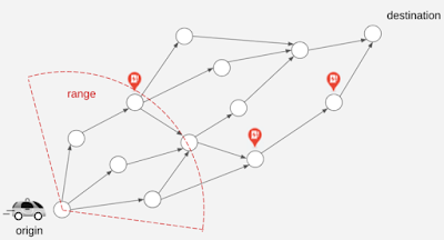
The EV can only travel a distance up to the illustrated range before needing to recharge. Different roads and different stations have different time costs. The goal is to optimize for the total trip time.

Today, we present a new approach for routing of EVs integrated into the latest release of Google Maps built into your car for participating EVs that reduces range anxiety by integrating recharging stations into the navigational route. Based on the battery level and the destination, Maps will recommend the charging stops and the corresponding charging levels that will minimize the total duration of the trip. To accomplish this we engineered a highly scalable solution for recommending efficient routes through charging stations, which optimizes the sum of the driving time and the charging time together.

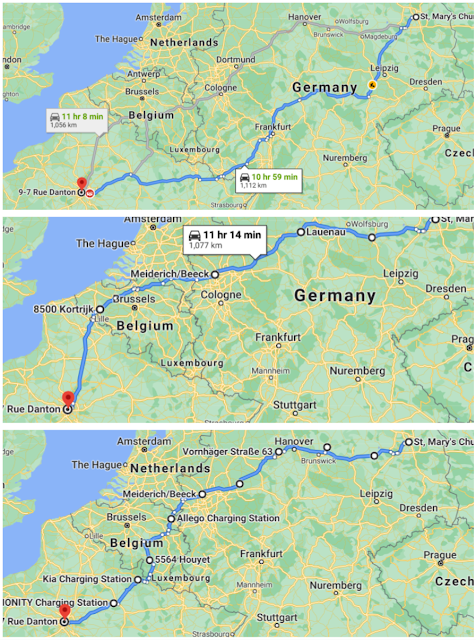
The fastest route from Berlin to Paris for a gas fueled car is shown in the top figure. The middle figure shows the optimal route for a 400 km range EV (travel time indicated – charging time excluded), where the larger white circles along the route indicate charging stops. The bottom figure shows the optimal route for a 200 km range EV.

Routing Through Charging Stations
A fundamental constraint on route selection is that the distance between recharging stops cannot be higher than what the vehicle can reach on a full charge. Consequently, the route selection model emphasizes the graph of charging stations, as opposed to the graph of road segments of the road network, where each charging station is a node and each trip between charging stations is an edge. Taking into consideration the various characteristics of each EV (such as the weight, maximum battery level, plug type, etc.) the algorithm identifies which of the edges are feasible for the EV under consideration and which are not. Once the routing request comes in, Maps EV routing augments the feasible graph with two new nodes, the origin and the destination, and with multiple new (feasible) edges that outline the potential trips from the origin to its nearby charging stations and to the destination from each of its nearby charging stations.

Routing using Dijkstra’s algorithm or A* on this graph is sufficient to give a feasible solution that optimizes for the travel time for drivers that do not care at all about the charging time, (i.e., drivers who always fully charge their batteries at each charging station). However, such algorithms are not sufficient to account for charging times. In this case, the algorithm constructs a new graph by replicating each charging station node multiple times. Half of the copies correspond to entering the station with a partially charged battery, with a charge, x, ranging from 0%-100%. The other half correspond to exiting the station with a fractional charge, y (again from 0%-100%). We add an edge from the entry node at the charge x to the exit node at charge y (constrained by y > x), with a corresponding charging time to get from x to y. When the trip from Station A to Station B spends some fraction (z) of the battery charge, we introduce an edge between every exit node of Station A to the corresponding entry node of Station B (at charge xz). After performing this transformation, using Dijkstra or A* recovers the solution.

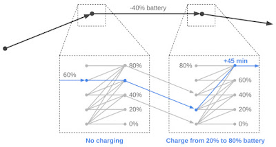
An example of our node/edge replication. In this instance the algorithm opts to pass through the first station without charging and charges at the second station from 20% to 80% battery.

Graph Sparsification
To perform the above operations while addressing range anxiety with confidence, the algorithm must compute the battery consumption of each trip between stations with good precision. For this reason, Maps maintains detailed information about the road characteristics along the trip between any two stations (e.g., the length, elevation, and slope, for each segment of the trip), taking into consideration the properties of each type of EV.

Due to the volume of information required for each segment, maintaining a large number of edges can become a memory intensive task. While this is not a problem for areas where EV charging stations are sparse, there exist locations in the world (such as Northern Europe) where the density of stations is very high. In such locations, adding an edge for every pair of stations between which an EV can travel quickly grows to billions of possible edges.

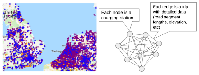
The figure on the left illustrates the high density of charging stations in Northern Europe. Different colors correspond to different plug types. The figure on the right illustrates why the routing graph scales up very quickly in size as the density of stations increases. When there are many stations within range of each other, the induced routing graph is a complete graph that stores detailed information for each edge.

However, this high density implies that a trip between two stations that are relatively far apart will undoubtedly pass through multiple other stations. In this case, maintaining information about the long edge is redundant, making it possible to simply add the smaller edges (spanners) in the graph, resulting in sparser, more computationally feasible, graphs.

The spanner construction algorithm is a direct generalization of the greedy geometric spanner. The trips between charging stations are sorted from fastest to slowest and are processed in that order. For each trip between points a and b, the algorithm examines whether smaller subtrips already included in the spanner subsume the direct trip. To do so it compares the trip time and battery consumption that can be achieved using subtrips already in the spanner, against the same quantities for the direct ab route. If they are found to be within a tiny error threshold, the direct trip from a to b is not added to the spanner, otherwise it is. Applying this sparsification algorithm has a notable impact and allows the graph to be served efficiently in responding to users’ routing requests.

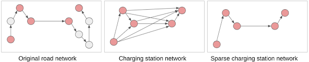
On the left is the original road network (EV stations in light red). The station graph in the middle has edges for all feasible trips between stations. The sparse graph on the right maintains the distances with much fewer edges.

Summary
In this work we engineer a scalable solution for routing EVs on long trips to include access to charging stations through the use of graph sparsification and novel framing of standard routing algorithms. We are excited to put algorithmic ideas and techniques in the hands of Maps users and look forward to serving stress-free routes for EV drivers across the globe!

Acknowledgements
We thank our collaborators Dixie Wang, Xin Wei Chow, Navin Gunatillaka, Stephen Broadfoot, Alex Donaldson, and Ivan Kuznetsov.

Categories
Misc

A Sense of Responsibility: Lidar Sensor Makers Build on NVIDIA DRIVE

When it comes to autonomous vehicle sensor innovation, it’s best to keep an open mind — and an open development platform. That’s why NVIDIA DRIVE is the chosen platform on which the majority of these sensors run. In addition to camera sensors, NVIDIA has long recognized that lidar is a crucial component to an autonomous Read article >

The post A Sense of Responsibility: Lidar Sensor Makers Build on NVIDIA DRIVE appeared first on The Official NVIDIA Blog.

Categories
Misc

NVIDIA Announces Nsight Graphics 2021.1

Nsight Graphics 2021.1 is available to download – check out this article to see what’s new.

Nsight Graphics 2021.1 is available to download.

We now provide you with the ability to set any key to be the capture shortcut. This new keybinding is supported for all activities, including GPU Trace. F11 is the default binding for both capture and trace, but if you prefer the old behavior, the original capture keybinding is still supported (when the ‘Frame Capture (Target) > Legacy Capture Chord’ setting is set to Yes).

You can now profile applications which use D3D12 or Vulkan strictly for compute tasks using the new ‘One-shot’ option in GPU Trace. Tools that generate normal maps or use DirectML for image upscaling can now be properly profiled and optimized.  To enable this, set the ‘Capture Type’ to ‘One-shot [Beta]’

While TraceRays/DispatchRays has been the common way to initiate ray generation, it’s now possible to ray trace directly from your compute shaders using DXR1.1 and the new Khronos Vulkan Ray Tracing extension. In order to support this new approach, we’ve added links to the acceleration structure data for applications that use RayQuery calls in compute shaders.  

It’s important to know how much GPU Memory you’re using and to keep this as low as possible in Ray Tracing applications. We’re now making this even easier for you by adding size information to the Acceleration Structure Viewer.

Finally, we’ve added the Nsight HUD to Windows Vulkan applications in all frame debugging capture states. Previously the HUD was only activated once an application was captured.

We’re always looking to improve our HUD so please make sure to give us any feedback you might have.

For more details on Nsight Graphics 2021.1, check out the release notes (link).

We want to hear from you! Please continue to use the integrated feedback button that lets you send comments, feature requests, and bugs directly to us with the click of a button. You can send feedback anonymously or provide an email so we can follow up with you about your feedback. Just click on the little speech bubble at the top right of the window.

Try out the latest version of Nsight Graphics today!

Khronos released the final Vulkan Ray Tracing extensions today. NVIDIA Vulkan beta drivers available for download. Welcome to the era of portable, cross-vendor, cross-platform ray tracing acceleration! 

And be sure to check out the final Vulkan Ray Tracing extensions from the Khronos Group as well!  

Categories
Misc

Certifiably Fast: Top OEMs Debut World’s First NVIDIA-Certified Systems Built to Crush AI Workloads

AI, the most powerful technology of our time, demands a new generation of computers tuned and tested to drive it forward. Starting today, data centers can get boot up a new class of accelerated servers from our partners to power their journey into AI and data analytics. Top system makers are delivering the first wave Read article >

The post Certifiably Fast: Top OEMs Debut World’s First NVIDIA-Certified Systems Built to Crush AI Workloads appeared first on The Official NVIDIA Blog.

Categories
Offsites

Stabilizing Live Speech Translation in Google Translate

The transcription feature in the Google Translate app may be used to create a live, translated transcription for events like meetings and speeches, or simply for a story at the dinner table in a language you don’t understand. In such settings, it is useful for the translated text to be displayed promptly to help keep the reader engaged and in the moment.

However, with early versions of this feature the translated text suffered from multiple real-time revisions, which can be distracting. This was because of the non-monotonic relationship between the source and the translated text, in which words at the end of the source sentence can influence words at the beginning of the translation.

Transcribe (old) — Left: Source transcript as it arrives from speech recognition. Right: Translation that is displayed to the user. The frequent corrections made to the translation interfere with the reading experience.

Today, we are excited to describe some of the technology behind a recently released update to the transcribe feature in the Google Translate app that significantly reduces translation revisions and improves the user experience. The research enabling this is presented in two papers. The first formulates an evaluation framework tailored to live translation and develops methods to reduce instability. The second demonstrates that these methods do very well compared to alternatives, while still retaining the simplicity of the original approach. The resulting model is much more stable and provides a noticeably improved reading experience within Google Translate.

Transcribe (new) — Left: Source transcript as it arrives from speech recognition. Right: Translation that is displayed to the user. At the cost of a small delay, the translation now rarely needs to be corrected.

Evaluating Live Translation
Before attempting to make any improvements, it was important to first understand and quantifiably measure the different aspects of the user experience, with the goal of maximizing quality while minimizing latency and instability. In “Re-translation Strategies For Long Form, Simultaneous, Spoken Language Translation”, we developed an evaluation framework for live-translation that has since guided our research and engineering efforts. This work presents a performance measure using the following metrics:

  • Erasure: Measures the additional reading burden on the user due to instability. It is the number of words that are erased and replaced for every word in the final translation.
  • Lag: Measures the average time that has passed between when a user utters a word and when the word’s translation displayed on the screen becomes stable. Requiring stability avoids rewarding systems that can only manage to be fast due to frequent corrections.
  • BLEU score: Measures the quality of the final translation. Quality differences in intermediate translations are captured by a combination of all metrics.

It is important to recognize the inherent trade-offs between these different aspects of quality. Transcribe enables live-translation by stacking machine translation on top of real-time automatic speech recognition. For each update to the recognized transcript, a fresh translation is generated in real time; several updates can occur each second. This approach placed Transcribe at one extreme of the 3 dimensional quality framework: it exhibited minimal lag and the best quality, but also had high erasure. Understanding this allowed us to work towards finding a better balance.

Stabilizing Re-translation
One straightforward solution to reduce erasure is to decrease the frequency with which translations are updated. Along this line, “streaming translation” models (for example, STACL and MILk) intelligently learn to recognize when sufficient source information has been received to extend the translation safely, so the translation never needs to be changed. In doing so, streaming translation models are able to achieve zero erasure.

The downside with such streaming translation models is that they once again take an extreme position: zero erasure necessitates sacrificing BLEU and lag. Rather than eliminating erasure altogether, a small budget for occasional instability may allow better BLEU and lag. More importantly, streaming translation would require retraining and maintenance of specialized models specifically for live-translation. This precludes the use of streaming translation in some cases, because keeping a lean pipeline is an important consideration for a product like Google Translate that supports 100+ languages.

In our second paper, “Re-translation versus Streaming for Simultaneous Translation”, we show that our original “re-translation” approach to live-translation can be fine-tuned to reduce erasure and achieve a more favorable erasure/lag/BLEU trade-off. Without training any specialized models, we applied a pair of inference-time heuristics to the original machine translation models — masking and biasing.

The end of an on-going translation tends to flicker because it is more likely to have dependencies on source words that have yet to arrive. We reduce this by truncating some number of words from the translation until the end of the source sentence has been observed. This masking process thus trades latency for stability, without affecting quality. This is very similar to delay-based strategies used in streaming methods such as Wait-k, but applied only during inference and not during training.

Neural machine translation often “see-saws” between equally good translations, causing unnecessary erasure. We improve stability by biasing the output towards what we have already shown the user. On top of reducing erasure, biasing also tends to reduce lag by stabilizing translations earlier. Biasing interacts nicely with masking, as masking words that are likely to be unstable also prevents the model from biasing toward them. However, this process does need to be tuned carefully, as a high bias, along with insufficient masking, may have a negative impact on quality.

The combination of masking and biasing, produces a re-translation system with high quality and low latency, while virtually eliminating erasure. The table below shows how the metrics react to the heuristics we introduced and how they compare to the other systems discussed above. The graph demonstrates that even with a very small erasure budget, re-translation surpasses zero-flicker streaming translation systems (MILk and Wait-k) trained specifically for live-translation.

System     BLEU     Lag
(seconds)
    Erasure
Re-translation
(Transcribe old)
    20.4     4.1     2.1
+ Stabilization
(Transcribe new)
    20.2     4.1     0.1
Evaluation of re-translation on IWSLT test 2018 Engish-German (TED talks) with and without the inference-time stabilization heuristics of masking and biasing. Stabilization drastically reduces erasure. Translation quality, measured in BLEU, is very slightly impacted due to biasing. Despite masking, the effective lag remains the same because the translation stabilizes sooner.
Comparison of re-translation with stabilization and specialized streaming models (Wait-k and MILk) on WMT 14 English-German. The BLEU-lag trade-off curve for re-translation is obtained via different combinations of bias and masking while maintaining an erasure budget of less than 2 words erased for every 10 generated. Re-translation offers better BLEU / lag trade-offs than streaming models which cannot make corrections and require specialized training for each trade-off point.

Conclusion
The solution outlined above returns a decent translation very quickly, while allowing it to be revised as more of the source sentence is spoken. The simple structure of re-translation enables the application of our best speech and translation models with minimal effort. However, reducing erasure is just one part of the story — we are also looking forward to improving the overall speech translation experience through new technology that can reduce lag when the translation is spoken, or that can enable better transcriptions when multiple people are speaking.