So let’s say I have 1 metric I want to monitor across the mode fitting process. So far, I’ve adapted the default CallBack function which allows me to get one single value for that given metric in each epoch. With this, I can save a time-series (just as with CSV logger) plot to check for the performance evolution but it doesn’t provide robustness results. Therefore, I would like to get the metric value for every sample in each epoch and save it, allowing me to get a time-series plot with a 95% confidence.
Hey, I am doing skin cancer classification with 9 classes, i am having a problem with overfitting as my train Accuracy can reach up to 90 with test acc=50 at best.
I have tried dropout, l2,l1 data augmentation lowering my network size, class weights, all it did was a longer training epoch with the same results as test acc never improved.
I am using cnn, is there another architect I can use? can I transfer this problem to “one vs all”?using TensorFlow ?
Hello I’m trying to make an image classifier which classifies given tomato plant leaf as [‘Tomato___Early_blight’, ‘Tomato___Septoria_leaf_spot’, ‘Tomato___healthy’]. I took the dataset from here It is already augmented and from that I took only Tomato plant leaf images and further reduced it to only three classes as mentioned before.
Here is my code
import tensorflow as tf
from tensorflow import keras
from tensorflow.keras.preprocessing.image import ImageDataGenerator
from tensorflow.keras.preprocessing.image import load_img, img_to_array
As you can see my model validation accuracy is good but its classifications are really bad even for the images from training dataset. How can I solve this problem .
Apologies if this information is readily available and I couldn’t find it. Would it be appropriate to set up a dedicated server strictly for tensorflow in a business environment? The goal would be classifying document imagines. The volume, I can only estimate, would be 1 to 4 million.
Recommender systems are the economic engine of the Internet. It is hard to imagine any other type of applications with more direct impact in our daily digital lives: Trillions of items to be recommended to billions of people. Recommender systems filter products and services among an overwhelming number of options, easing the paradox of choice … Continued
Recommender systems are the economic engine of the Internet. It is hard to imagine any other type of applications with more direct impact in our daily digital lives: Trillions of items to be recommended to billions of people. Recommender systems filter products and services among an overwhelming number of options, easing the paradox of choice that most users face.
Embeddings play a critical role in modern DL-based recommender architectures, encoding individual information for billions of entities (users, products, and their characteristics). As the amount of data increases, so does the size of the embedding tables, now spanning multiple GBs to TBs. There are unique challenges in training this type of DL system, with its huge embedding tables with sparse access patterns spanning potentially multiple GPUs, if not nodes.
This post focuses on how the NVIDIA Merlin recommendation system framework addresses these challenges and introduces an optimized embedding implementation that is up to 8x more performant than other frameworks’ embedding layers. This optimized implementation is also made available as a TensorFlow plugin that works seamlessly with TensorFlow and acts as a convenient drop-in replacement for the TensorFlow native embedding layers.
Embeddings
Embedding is a machine learning technique that represents each object of interest (users, products, categories, and so on) as a dense numerical vector. Embedding tables are hence nothing other than a specific type of key-value store, with keys being the ID used to uniquely identify objects and values being vectors of real numbers.
Embedding is a key building block in modern DL recommender systems, typically lying immediately after the input layer and before “feature interaction” and dense layers. Embedding layers are learned from data and end-to-end training, just like other layers of a deep neural network. It is the embedding layers that differentiate DL recommender models from other types of DL workloads: they contribute an enormous number of parameters to the model but require little to no computation, while the compute-intensive dense layers have a much smaller number of parameters.
Take a specific example: The original Wide and Deep model has several dense layers of size [1024, 512, 256], hence only a few million parameters, while its embedding layers can have billions of entries, and multiple billions of parameters. This contrasts with, for example, a BERT model architecture popular in the NLP domain, where the embedding layer has only tens of thousands of entries amounting to several millions of parameters, but the dense feed-forward and attention layers consist of several hundreds of millions of parameters. This differentiation also leads to another observation: the amount of compute per byte of input data for DL recommender networks is typically much smaller compared to other types of DL models.
Why optimizing embeddings matters for recommender workflows
To understand why optimization of the embedding layer and related operations matters, here are the challenges of training embeddings: size and access speed.
Size
With online platforms and services acquiring hundreds of millions to even billions of users, and with the number of unique products on offer reaching billions, it is not surprising that embedding tables are increasing in size.
Naturally, it presents a significant challenge fitting a TB-scale model on a single node of compute, let alone a single compute accelerator. For reference, the largest NVIDIA A100 GPU is currently equipped with 80 GB of HBM.
Access speed
Training recommender systems is inherently a memory bandwidth-intensive task. This is because each training sample or batch usually involves a small number of entities in the embedding tables. These entries must be retrieved to calculate the forward pass, then updated in the backward pass.
The CPU main memory has high capacity but limited bandwidth, with high-end models typically in the high tens of GB/s range. The GPU, on the other hand, has limited memory capacity but high bandwidth. An NVIDIA A100 80-GB GPU offers 2 TB/s of memory bandwidth.
Solutions
These challenges have been addressed in different ways. For example, keeping the entire embedding table on main memory solves the size issue. However, it most often results in extremely slow training throughput that is often dwarfed by the amount and velocity of new data, forbidding the system to be retrained in a timely manner.
Alternatively, the embedding can be carefully spread across multiple GPUs and multiple nodes, only to be bogged down by the communication bottleneck, resulting in sustained severe GPU-compute under-utilization and training performance just on par with pure CPU training.
The embedding layer is one of the major bottlenecks in recommender systems. Optimizing the embedding layer is key to unlocking the GPU’s high compute throughput.
In the next section, we discuss how the NVIDIA Merlin HugeCTR recommender framework solves the challenges of large-scale embeddings, by using NVIDIA technologies such as GPUDirect remote direct memory access (RDMA), NVIDIA Collective Communications Library (NCCL), NVLink, and NVSwitch. It unlocks both the high-compute and high-bandwidth capacity of the GPU, while addressing the memory capacity problem with out-of-the-box, multi-GPU, multinode support and model parallelism.
Overview of NVIDIA Merlin HugeCTR embeddings
NVIDIA Merlin addresses the challenges of training large-scale recommender systems. It’s an end-to-end recommender framework that accelerates all phases of recommendation system development, from data preprocessing to training and inference. NVIDIA Merlin HugeCTR is an open-source, recommender system, dedicated DL framework. In this post, we focus on one specific aspect of HugeCTR: embedding optimization.
There are two ways to leverage the embedding optimization work in HugeCTR:
Using the native NVIDIA Merlin HugeCTR framework for your training and inference workloads
Using the NVIDIA Merlin HugeCTR TensorFlow plugin, which is designed to work seamlessly with TensorFlow
Native HugeCTR embedding optimization
To overcome the embedding challenges and enable faster training, HugeCTR implemented its own embedding layer, which includes a GPU-accelerated hash table, efficient sparse optimizers implemented in a memory-saving manner, and various embedding distribution strategies. It harnesses NCCL as its inter-GPU communication primitives.
Built with scalability in mind, HugeCTR supports model parallelism for the embedding layer by default. The embedding tables are distributed across the available GPUs and nodes. The dense layers, on the other hand, employ data parallelism (Figure 1).
Figure 1. Embedding layer parallelism in HugeCTR
The Tencent recommendation team is one of the first adopters of the native HugeCTR framework, making heavy use of its native embedding layers. In a recent interview, Xiangting Kong, lead of the Tencent Advertising and Deep Learning Platform said, “HugeCTR, as a recommendation training framework, is integrated into the [Tencent] advertising recommendation training system to make the update frequency of model training faster, and more samples can be trained to improve online effects.”
HugeCTR TensorFlow plugin
All components of the NVIDIA Merlin framework are open-source and designed to be interoperable with the larger deep learning and data science ecosystem. Our long-term vision is to accelerate recommendation workloads on the GPU, regardless of your preferred framework. The HugeCTR TensorFlow embedding plugin was created as a step towards realizing this goal.
At a high level, the TensorFlow embedding plugin is designed by leveraging many of the same embedding optimization techniques that were employed for the native HugeCTR embedding layer. In particular, this would be the GPU hash table and NCCL under the hood for inter-GPU communication.
The HugeCTR embedding plugin is designed to work conveniently and seamlessly with TensorFlow as a drop in replacement for the TensorFlow-native embedding layers, such as tf.nn.embedding_lookup and tf.nn.embedding_lookup_sparse. It also offers advanced features out of the box, such as model parallelism that distributes the embedding tables over multiple GPUs.
Here’s how to make use of the TensorFlow embedding plugin. The full example is available at the HugeCTR repository, where we also provide a full benchmarking notebook for reproducing the performance figures.
The most convenient way to access the HugeCTR embedding plugin is through using the NGC NVIDIA Merlin TensorFlow training Docker image, in which it is precompiled and installed, along with other components of the NVIDIA Merlin framework, as well as TensorFlow. The most up-to-date version can be pulled directly from the HugeCTR repository, compiled and installed on the fly. When TensorFlow is updated, the plugin must also be recompiled for the newly installed TensorFlow version.
For comparison, here’s how the native TensorFlow embedding layers are used. First, you initialize a 2D-array variable to hold the value of the embeddings. Then, use tf.nn.embedding_lookup to look up the embedding value corresponding to a list of IDs.
embedding_var = tf.Variable(initial_value=initial_value, dtype=tf.float32, name='embedding_variables')

@tf.function
def _train_step(inputs, labels):
    emb_vectors = tf.nn.embedding_lookup([self.embedding_var], inputs)
    ...

for i, (inputs, labels) in enumerate(dataset):
    _train_step(inputs)
In the same fashion, the HugeCTR embedding plugin can be employed. First, you initialize an embedding layer. Next, this embedding layer is used to look up the corresponding embedding values for a list of IDs.
import sparse_operation_kit as sok

emb_layer = sok.All2AllDenseEmbedding(max_vocabulary_size_per_gpu,
                                      embedding_vec_size,
                                      slot_num, nnz_per_slot)

@tf.function
def _train_step(inputs, labels):
    emb_vectors = emb_layer(inputs)
    ...

for i, (inputs, labels) in enumerate(dataset):
    _train_step(inputs)
The HugeCTR embedding plugin is designed to work seamlessly with TensorFlow, including other layers and optimizers such as Adam and sgd. Before TensorFlow v2.5, the Adam optimizer was a CPU-based implementation.
To fully realize the potential of the HugeCTR embedding plugin, we also provide a GPU-based plugin_adam version in sok.optimizers.Adam. Starting from TensorFlow v2.5, the standard Adam optimizer tf.keras.optimizers.Adam, which now comes with a GPU implementation, can be used with similar accuracy and performance.
Performance benchmark
In this section, we showcase the performance of the HugeCTR TensorFlow embedding plugin through synthetic and real use cases.
Synthetic data
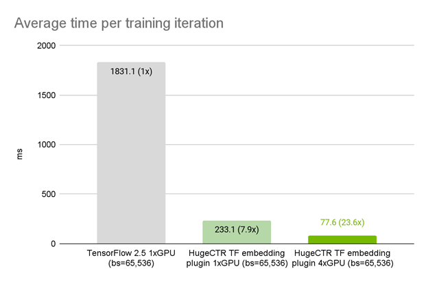
In this example, we use a synthetic dataset with 100 feature fields, each with 10 lookups, and a vocabulary size of 8192. The recommender model is an MLP with six layers, each of size 1024. Using the exact model architecture, optimizer, and data loader in TensorFlow, we observed that on 1x A100 GPU, the HugeCTR embedding plugin improves the average iteration time by 7.9x compared to the native TensorFlow embedding layer (Figure 2).
When being strong-scaled from one to four A100 GPUs, we observed a total speedup of 23.6x. This benefit of multi-GPU scaling is provided by the HugeCTR embedding plugin by default. Under the hood, the embedding plugin automatically distributes the table corresponding to feature fields on to the available GPUs in a model parallel fashion. This contrasts with the native TensorFlow embedding layer, where a significant extra effort is required for distributed model-parallel multi-GPU training. The TensorFlow distribution strategies, MirroredStrategy and MultiWorkerMirroredStrategy, are both designed to do data-parallel synchronized training.
Figure 2. HugeCTR TensorFlow embedding plugin performance on NVIDIA DGX A100 80GB on synthetic dataset
Real use case: Meituan recommender systems
The Meituan recommender systems team is one of the first teams to adopt the HugeCTR TensorFlow plugin with great success. At first, the team optimized their training framework based on CPU, but as their models became more and more complex, it was difficult to optimize the training framework more deeply. Now, Meituan is working on integrating NVIDIA HugeCTR into their training system based on A100 GPUs.
“A single server with 8x A100 GPUs can replace hundreds of workers in the CPU based training system. The cost is also greatly reduced. This is a preliminary optimization result, and there is still much room to optimize in the future,” shared Jun Huang, senior technical expert at Meituan.
Meituan used DIEN as the recommendation model. The total number of embedding parameters is tens of billions, and there are thousands of feature fields in each sample. As the range of input features is not fixed and unknown in advance, the team uses hash tables to uniquely identify each input feature before feeding into an embedding layer.
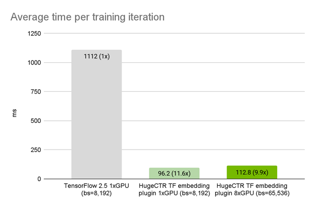
Using the exact model architecture, optimizer, and data loader in TensorFlow, we observed that on a single A100 GPU, the HugeCTR embedding plugin achieved a 11.5x speedup compared to the original TensorFlow embedding. With weak scaling, the iteration time on 8x A100 GPUs only increased slightly to 1.17x that of 1x A100 GPU (Figure 3).
Figure 3. HugeCTR TensorFlow embedding plugin performance on NVIDIA DGX A100 80GB on Meituan data
Conclusion
The HugeCTR TensorFlow embedding plugin is available today from the HugeCTR GitHub repository, as well as from the NGC NVIDIA Merlin TensorFlow container. If you are a TensorFlow user looking to build and deploy large-scale recommender systems with large embedding tables, the HugeCTR TensorFlow plugin is a great effortless drop-in replacement for TensorFlow embedding lookup layers.
Try it out to see the full potential of your GPUs unlocked. If you feel that you need even more performance and optimization, then the full-fledged native HugeCTR framework might be the next thing that you want to try.
Developers are encouraged to download, explore, and evaluate experimental AI models for Deep Learning Super Sampling.
Today, NVIDIA is enabling developers to explore and evaluate experimental AI models for Deep Learning Super Sampling (DLSS). Developers can download experimental Dynamic-link libraries (DLLs), test how the latest DLSS research enhances their games, and provide feedback for future improvements.
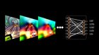
NVIDIA DLSS is a deep learning neural network that boosts frame rates and generates beautiful, sharp images for your games. It gives you the performance headroom to maximize ray tracing settings and increase output resolution.
Powered by dedicated AI processors on NVIDIA RTX GPUs called Tensor Cores, NVIDIA DLSS technology has already been adopted and implemented in over 100 games and applications. These include gaming franchises such as Cyberpunk, Call of Duty, DOOM, Fortnite, LEGO, Minecraft,Rainbow Six, and Red Dead Redemption, with support coming soon for Battlefield 2042.
One of the key advantages of a deep learning approach to super sampling is that the AI model can continuously improve through ongoing training on the NVIDIA supercomputer. In fact, each major production release of DLSS has delivered better image quality across wider ranges of games and applications.
We are inviting the developer community to test the latest experimental DLSS models straight off the supercomputer, and provide us feedback. The experimental DLLs contain improvements that show promise of image quality, but have not yet been thoroughly validated. Your early input is important to helping us push the state of the art in AI graphics technology.
Get Started Now
Go to the NVIDIA developer page to see the DLLs available for testing. Getting started is seamless—download the DLL package of your choice, replace the existing DLL in your game, and then simply run.
Learn more about NVIDIA game developer offerings >>
Learn how NVDashboard in Jupyter Lab is a great open-source package to monitor system resources for all GPU and RAPIDS users to achieve optimal performance and day to day model and workflow development.
This post was originally published on the RAPIDS AI blog here.
Introduction
NVDashboard is an open-source package for the real-time visualization of NVIDIA GPU metrics in interactive Jupyter Lab environments. NVDashboard is a great way for all GPU users to monitor system resources. However, it is especially valuable for users of RAPIDS, NVIDIA’s open-source suite of GPU-accelerated data-science software libraries.
Given the computational intensity of modern data-science algorithms, there are many cases in which GPUs can offer game-changing workflow acceleration. To achieve optimal performance, it is absolutely critical for the underlying software to use system resources effectively. Although acceleration libraries (like cuDNN and RAPIDS) are specifically designed to do the heavy lifting in terms of performance optimization, it can be very useful for both developers and end-users to verify that their software is actually leveraging GPU resources as intended. While this can be accomplished with command-line tools like nvidia-smi, many professional data scientists prefer to use interactive Jupyter notebooks for day-to-day model and workflow development.
Figure 1: The NVDashboard Jupyter-Lab extension in action. The GPU dashboards are shown along the right-hand side of the screen, while two dask-labextension dashboards are shown on the bottom left) [GIF].
As illustrated in Fig. 1, NVDashboard enables Jupyter notebook users to visualize system hardware metrics within the same interactive environment they use for development. Supported metrics include:
GPU-compute utilization
GPU-memory consumption
PCIe throughput
NVLink throughput
The package is built upon a Python-based dashboard server, which support the Bokeh visualization library to display and update figures in real time[1] . An additional Jupyter-Lab extension embeds these dashboards as movable windows within an interactive environment. Most GPU metrics are collected through PyNVML, an open-source Python package composing wrappers for the NVIDIA Management Library (NVML). For this reason, the available dashboards can be modified/extended to display any queryable GPU metrics accessible through NVML.
Using NVDashboard
The nvdashboard package is available on PyPI, and consists of two basic components:
Bokeh Server: The server component leverages the wonderful Bokeh visualization library to display and update GPU-diagnostic dashboards in real time. The desired hardware metrics are accessed with PyNVML, an open-source python package composing wrappers for the NVIDIA Management Library (NVML). For this reason, NVDashboard can be modified/extended to display any queryable GPU metrics accessible through NVML, easily from Python.
Jupyter-Lab Extension: The Jupyter-Lab extension makes embedding the GPU-diagnostic dashboards as movable windows within an interactive Jupyter-Lab environment.
The Jupyter Lab Extension
The practice of directly querying hardware metrics is often the best way to validate efficient run-time behavior, and this is especially true for interactive Jupyter-notebook users. In this case, the development process is often iterative, and improper GPU utilization results in huge productivity losses. As shown in Fig. 1, NVDashboard makes visualizing resource utilization easy for Jupyter-Lab users right alongside their code.
To install both the server and client-side components, run the following in a terminal:
After NVDashborad is installed, a “GPU Dashboards” menu should be visible along the left-hand side of your Jupyter-Lab environment (see Fig. 2). Clicking on one of these buttons automatically adds a movable window, with a real-time display of the desired dashboard.
Figure 2: Main menu for the Jupyter-Lab extension.
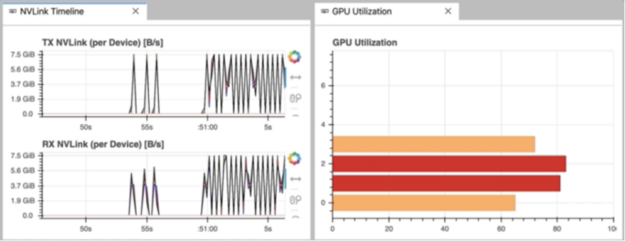
It is important to clarify that NVDashboard automatically monitors the GPU resources for the entire machine, not only those being used by the local Jupyter environment. The Jupyter-Lab eExtension can certainly be used for non-iPython/notebook development. For example, in Fig. 3, the “NVLink Timeline” and “GPU Utilization” dashboards are being used within a Jupyter-Lab environment to monitor a multi-GPU deep-learning workflow executed from the command line.
Figure 3: The “NVLink Timeline” dashboard being used with Jupyter Lab [GIF].
The Boker server
While the Jupyter-Lab extension is certainly ideal for fans of iPython/notebook-based development, other GPU users can also access the dashboards using a sandalone Bokeh server. This is accomplished by running.
$ python -m jupyterlab_nvdashboard.server
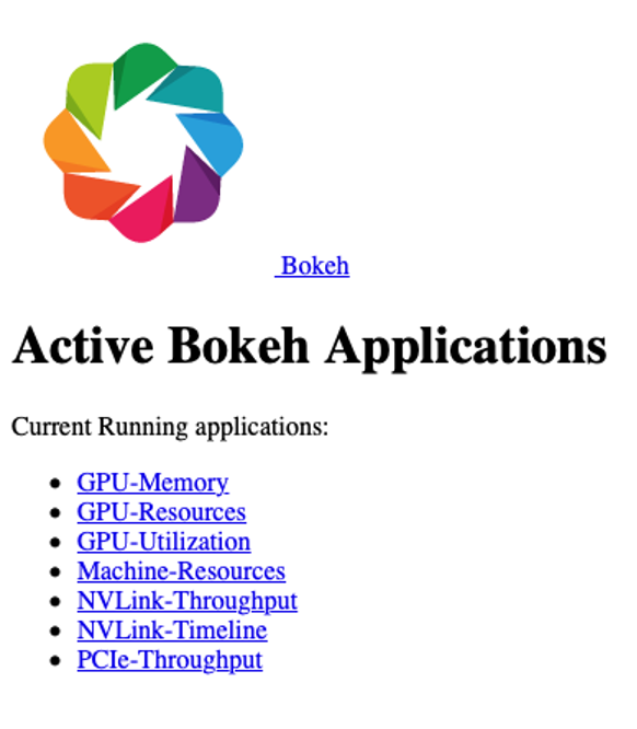
After starting the Bokeh server, the GPU dashboards are accessed by opening the appropriate url in a standard web browser (for example, http://:). As shown in Fig. 4, the main menu lists all dashboards available in NVDashboard.
Figure 4: The main menu for the Bokeh-server component of NVDashboard.
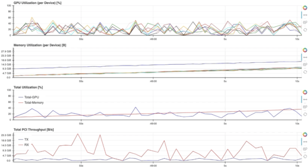
For example, selecting the “GPU-Resources” link opens the dashboard shown in Fig. 5, which summarizes the utilization of various GPU resources using aligned timeline plots.
Figure 5: The “GPU Resources” dashboard being used outside of Jupyter Lab [GIF].
To use NVDashboard in this way, only the pip-installation step is needed (the lab extension installation step can be skipped):
$ pip install jupyterlab-nvdashboard
Alternatively, one can also clone the jupyterlab-nvdashboard repository, and simply execute the server.py script (for example, python jupyterlab_nvdashboard/server.py ).
Implementation details
The existing nvdashboard package provides a number of useful GPU-resource dashboards. However, it is fairly straightforward to modify existing dashboards and/or create completely new ones. In order to do this, you simply need to leverage PyNVML and Bokeh.
PyNVML dasic
PyNVML is a python wrapper for the NVIDIA Management Library (NVML), which is a C-based API for monitoring and managing various states of NVIDIA GPU devices. NVML is directly used by the better-known NVIDIA System Management Interface (nvidia-smi). According to the NVIDIA developer site, NVML provides access to the following query-able states (in additional to modifiable states not discussed here):
ECC error counts: Both correctable single bit and detectable double bit errors are reported. Error counts are provided for both the current boot cycle and for the lifetime of the GPU.
GPU utilization: Current utilization rates are reported for both the compute resources of the GPU and the memory interface.
Active compute process: The list of active processes running on the GPU is reported, along with the corresponding process name/id and allocated GPU memory.
Clocks and PState: Max and current clock rates are reported for several important clock domains, as well as the current GPU performance state.
Temperature and fan speed: The current core GPU temperature is reported, along with fan speeds for non-passive products.
Power management: For supported products, the current board power draw and power limits are reported.
Identification: Various dynamic and static information is reported, including board serial numbers, PCI device ids, VBIOS/Inforom version numbers and product names.
Although several different python wrappers for NVML currently exist, we use the PyNVML package hosted by GoAi on GitHub. This version of PyNVML uses ctypes to wrap most of the NVML C API. NVDashboard utilizes only a small subset of the API needed to query real-time GPU-resource utilization, including:
nvmlInit(): Initialize NVML. Upon successful initialization, the GPU handles are cached to lower the latency of data queries during active monitoring in a dashboard.
nvmlShutdown(): Finalize NVML
nvmlDeviceGetCount(): Get the number of available GPU devices
nvmlDeviceGetHandleByIndex(): Get a handle for a device (given an integer index)
nvmlDeviceGetMemoryInfo(): Get a memory-info object (given a device handle)
nvmlDeviceGetUtilizationRates(): Get a utilization-rate object (given a device handle)
nvmlDeviceGetPcieThroughput(): Get a PCIe-throughput object (given a device handle)
nvmlDeviceGetNvLinkUtilizationCounter(): Get an NVLink utilization counter (given a device handle and link index)
In the current version of PyNVML, the python function names are usually chosen to exactly match the C API. For example, to query the current GPU-utilization rate on every available device, the code would look something like this:
In [1]: from pynvml import *
In [2]: nvmlInit()
In [3]: ngpus = nvmlDeviceGetCount()
In [4]: for i in range(ngpus):
…: handle = nvmlDeviceGetHandleByIndex(i)
…: gpu_util = nvmlDeviceGetUtilizationRates(handle).gpu
…: print(‘GPU %d Utilization = %d%%’ % (i, gpu_util))
…:
GPU 0 Utilization = 43%
GPU 1 Utilization = 0%
GPU 2 Utilization = 15%
GPU 3 Utilization = 0%
GPU 4 Utilization = 36%
GPU 5 Utilization = 0%
GPU 6 Utilization = 0%
GPU 7 Utilization = 11%
Note that, in addition to the GitHub repository, PyNVML is also hosted on PyPI and Conda Forge.
Dashboard Code
In order to modify/add a GPU dashboard, it is only necessary to work with two files (jupyterlab_bokeh_server/server.py and jupyterlab_nvdashboard/apps/gpu.py). Most of the PyNVML and bokeh code needed to add/modify a dashboard will be in gpu.py. It is only necessary to modify server.py in the case that you are adding or changing a menu/display name. In this case, the new/modified name must be specified in routes dictionary (with the key being the desired name, and the value being the corresponding dashboard definition):
In order for the server to constantly refresh the PyNVML data used by the bokeh applications, we use bokeh’s ColumnDataSource class to define the source of data in each of our plots. The ColumnDataSource class allows an update function to be passed for each type of data, which can be called within a dedicated callback function (cb) for each application. For example, the existing gpu application is defined like this:
Note that the real-time update of PyNVML GPU-utilization data is performed within the source.data.update() call. With the necessary ColumnDataSource logic in place, the standard GPU definition (above) can be modified in many ways. For example, swapping the x and y axes, specifying a different color palette, or even changing the figure from an hbar to something else entirely.
Users should feel free to open a pull request to contribute valuable improvements/additions — Community engagement is certainly encouraged!
Jupyter Lab extension code
In order to package this up as a Jupyter Lab extension we need our bokeh server to be run when Jupyter Lab starts. We can do this by adding jupyter-server-proxy as a dependency and registering an entrypoint in our setup.py:
This results in Jupyter Lab launching our bokeh server when it is run and proxying traffic through from /nvdashboard to it.
Then we can write a JavaScript frontend extension for Jupyter Lab which adds a sidebar menu with a list of dashboards which are opened as IFrames in new tabs in the interface. This is installed by running jupyter labextension install jupyterlab-nvdashboard.
There is also a custom Bokeh server endpoint in the Python side of things which serves a list of all the available dashboards and their URLs as a json file at /nvdashboard/index.json. The front end can use this json file to populate the menu automatically. This means that if we want to add any new dashboards we can do everything on the Python side by adding new Bokeh apps and the Jupyter Lab extension will pick them up automatically.
I was looking through the documentation and its currently not clear, in some sources it’s said that subgraphs are not supported, but the tensorflow page says unidirectional lstms are supported, and I am confused, can anyone point me to TFLM implementation of an LSTM?


")
 Recommender systems are the economic engine of the Internet. It is hard to imagine any other type of applications with more direct impact in our daily digital lives: Trillions of items to be recommended to billions of people. Recommender systems filter products and services among an overwhelming number of options, easing the paradox of choice …
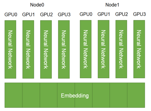
 Developers are encouraged to download, explore, and evaluate experimental AI models for Deep Learning Super Sampling.
 Learn how NVDashboard in Jupyter Lab is a great open-source package to monitor system resources for all GPU and RAPIDS users to achieve optimal performance and day to day model and workflow development.
