Speech is the most natural form of human communication. So, it’s not surprising that we’ve always wanted to interact with and command machines by voice. However, for conversational AI to provide a seamless, natural, and human-like experience, it needs to be trained on large amounts of data representative of the problem the model is trying … Continued
Speech is the most natural form of human communication. So, it’s not surprising that we’ve always wanted to interact with and command machines by voice. However, for conversational AI to provide a seamless, natural, and human-like experience, it needs to be trained on large amounts of data representative of the problem the model is trying to solve. The difficulty for machine learning teams is the scarcity of this high-quality, domain-specific data.
Companies are trying to solve this problem and accelerate the widespread adoption of conversational AI with innovative solutions that guarantee the scalability and internationality of models. NVIDIA and DefinedCrowd are two such companies. By providing machine learning engineers with a model-building toolkit and high-quality training data respectively, NVIDIA and DefinedCrowd integrate to create world-class AI simply, easily, and quickly.
DefinedCrowd, a one-stop shop for AI training data
I am the director of machine learning at DefinedCrowd, and our core business is providing high-quality AI training data to companies building world-class AI solutions. Our customers can access this data through DefinedData, an online marketplace of off-the-shelf AI training data available in multiple languages, domains, and recording types.
If you can’t find what you’re looking for in DefinedData, our workflows can serve as standalone or end-to-end data services to build any speech– or text-enabled AI architecture from scratch, to improve solutions already developed, or to evaluate models in production, all with the DefinedCrowd quality guarantee.
Creating conversational AI applications the easy way
NVIDIA NeMo is a toolkit built by NVIDIA for creating conversational AI applications. This toolkit includes collections of pretrained modules for automatic speech recognition (ASR), natural language processing (NLP), and text-to-speech (TTS), enabling researchers and data scientists to easily compose complex neural network architectures and focus on designing their applications.
NeMo and DefinedCrowd integration
Here’s how to connect DefinedCrowd speech workflows to train and improve an ASR model using NVIDIA NeMo. The code can also be accessed on this Google Colab link.
Step 1: Install NeMo Toolkit and dependencies
# First, install NeMo Toolkit and dependencies to run this notebook
!apt-get install -y libsndfile1 ffmpeg
!pip install Cython

## Install NeMo dependencies in the correct versions
!pip install torchtext==0.8.0 torch==1.7.1 pytorch-lightning==1.2.2

## Install NeMo
!python -m pip install nemo_toolkit[all]==1.0.0b3
Step 2: Obtain data using the DefinedCrowd API
Here’s how to connect to the DefinedCrowd API to obtain speech collected data. For more information, see DefinedCrowd API (v2).
# For the demo, use a sandbox environment
auth_url = "https://sandbox-auth.definedcrowd.com"
api_url = "https://sandbox-api.definedcrowd.com"

# These variables should be obtained at the DefinedCrowd Enterprise Portal for your account.
client_id = ""
client_secret = ""
project_id = ""
Authentication
payload = {
    "client_id": client_id,
    "client_secret": client_secret,
    "grant_type": "client_credentials",
    "scope": "PublicAPIv2",
}
files = []
headers = {}

# request the Auth 2.0 access token
response = requests.request(
    "POST", f"{auth_url}/connect/token", headers=headers, data=payload, files=files
)
if response.status_code == 200:
    print("Authentication success!")
    access_token = response.json()["access_token"]
else:
    print("Authentication Failed")
Authentication success!
List of deliverables
# GET /projects/{project-id}/deliverables
headers = {"Authorization": "Bearer " + access_token}
response = requests.request(
    "GET", f"{api_url}/projects/{project_id}/deliverables", headers=headers
)

if response.status_code == 200:
    # Pretty print the response
    print(json.dumps(response.json(), indent=4))

    # Get the first deliverable ID
    deliverable_id = response.json()[0]["id"]

[
    {
        "projectId": "eb324e45-c4f9-41e7-b5cf-655aa693ae75",
        "id": "258f9e15-2937-4846-b9c3-3ae1164b7364",
        "type": "Flat",
        "fileName": "data_Flat_eb324e45-c4f9-41e7-b5cf-655aa693ae75_258f9e15-2937-4846-b9c3-3ae1164b7364_2021-03-22-14-34-37.zip",
        "createdTimestamp": "2021-03-22T14:34:37.8037259",
        "isPartial": false,
        "downloadCount": 2,
        "status": "Downloaded"
    }
]
Final deliverable for speech data collection
# Name to give to the deliverable file
filename = "scripted_monologue_en_GB.zip"

# GET /projects/{project-id}/deliverables/{deliverable-id}/download
headers = {"Authorization": "Bearer " + access_token}
response = requests.request(
    "GET",
    f"{api_url}/projects/{project_id}/deliverables/{deliverable_id}/download/",
    headers=headers,
)

if response.status_code == 200:
    # save the deliverable file
    with open(filename, "wb") as fp:
        fp.write(response.content)
    print("Deliverable file saved with success!")
Deliverable file saved with success!
# Extract the contents from the downloaded file
!unzip  scripted_monologue_en_GB.zip &> /dev/null
!rm -f en-gb_single-scripted_Dataset.zip
Step 3: Analyze the speech dataset
Here’s how to analyze the data received from DefinedCrowd. The data is built of scripted speech data collected by the DefinedCrowd Neevo platform from several speakers in the UK (crowd members from DefinedCrowd).
Each row of the dataset contains information about the speech prompt, crowd member, device used, and the recording. The following data is found with this delivery:
- Recording:
- RecordingId
- PromptId
- Prompt
- Audio File:
- RelativeFileName
- Duration
- SampleRate
- BitDepth
- AudioCommunicationBand
- RecordingEnvironment
- Crowd Member:
- SpeakerId
- Gender
- Age
- Accent
- LivingCountry
- Recording Device:
- Manufacturer
- DeviceType
- Domain
This data can be used for multiple purposes, but in this tutorial, I use it for improving an existent ASR model for British speakers.
import pandas as pd

# Look in the metadata file
dataset = pd.read_csv("metadata.tsv", sep="t", index_col=[0])

# Check the data for the first row
dataset.iloc[0]

RecordingId                               165559628
PromptId                                   64977250
RelativeFileName                Audio/165559628.wav
Prompt                    The Avengers' extinction.
Duration                               00:00:02.815
SpeakerId                                    128209
Gender                                       Female
Age                                              26
Manufacturer                                  Apple
DeviceType                                iPhone 6s
Accent                                      Suffolk
Domain                                      generic
SampleRate                                    16000
BitDepth                                         16
AudioCommunicationBand                    Broadband
LivingCountry                        United Kingdom
Native                                         True
RecordingEnvironment                         silent
Name: 0, dtype: object

# How many rows do you have?
len(dataset)
50000
# Check some examples from the dataset
import librosa
import IPython.display as ipd

for index, row in dataset.sample(4, random_state=1).iterrows():

    print(f"Prompt: {dataset.iloc[index].Prompt}")
    audio_file = dataset.iloc[index].RelativeFileName

    # Load and listen to the audio file
    audio, sample_rate = librosa.load(audio_file)
    ipd.display(ipd.Audio(audio, rate=sample_rate))
For audio samples, see the DefinedCrowd x NeMo – ASR Training tutorial on Google Colab.
Step 4: Prepare the data
After downloading the speech data from DefinedCrowd API, you must adapt it for the format expected by NeMo for ASR training. For this, you create manifests for the training and evaluation data, including each audio file’s metadata.
NeMo requires that you adapt the data to a particular manifest format. Each line corresponding to one audio sample, so the line count equals the number of samples represented by the manifest. A line must contain the path to an audio file, the corresponding transcript, and the audio sample duration. For example, here is what one line might look like in a NeMo-compatible manifest:
{"audio_filepath": "path/to/audio.wav", "duration": 3.45, "text": "this is a nemo tutorial"}
For the creation of the manifest, also standardize the transcripts.
import os

# Function to build a manifest
def build_manifest(dataframe, manifest_path):
    with open(manifest_path, "w") as fout:
        for index, row in dataframe.iterrows():
            transcript = row["Prompt"]

            # The model uses lowercased data for training/testing
            transcript = transcript.lower()

            # Removing linguistic marks (they are not necessary for this demo)
            transcript = (
                transcript.replace("", "")
                .replace("", "")
                .replace("[b_s/]", "")
                .replace("[uni/]", "")
                .replace("[v_n/]", "")
                .replace("[filler/]", "")
                .replace('"', "")
                .replace("[n_s/]", "")
            )

            audio_path = row["RelativeFileName"]

            # Get the audio duration
            try:
                duration = librosa.core.get_duration(filename=audio_path)
            except Exception as e:
                print("An error occurred: ", e)

            if os.path.exists(audio_path):
                # Write the metadata to the manifest
                metadata = {
                    "audio_filepath": audio_path,
                    "duration": duration,
                    "text": transcript,
                }
                json.dump(metadata, fout)
                fout.write("n")
            else:
                continue
Step 5: Train and test splits
To test the quality of the model, you must reserve some data for model testing. Evaluate the model performance on this data.
import json
from sklearn.model_selection import train_test_split
# Split 10% for testing (500 prompts) and 90% for training (4500 prompts)
trainset, testset = train_test_split(dataset, test_size=0.1, random_state=1)
# Build the manifests
build_manifest(trainset, "train_manifest.json")
build_manifest(testset, "test_manifest.json")
Step 6: Configure the model
Here’s how to use the QuartzNet15x5 model as a base model for fine-tuning with the data. To improve the recognition of the dataset, benchmark the model performance on the base model and later, on the fine-tuned version. Some of the following functions were retrieved from the Nemo Tutorial on ASR.
# Import Nemo and the functions for ASR
import torch
import nemo
import nemo.collections.asr as nemo_asr
import logging
from nemo.utils import _Logger
# Set up the log level by NeMo
logger = _Logger()
logger.set_verbosity(logging.ERROR)
Step 7: Set training parameters
For training, NeMo uses a Python dictionary as data structure to keep all the parameters. For more information, see the NeMo ASR Config User Guide.
For this tutorial, load a preexisting file with the standard ASR configuration and change only the necessary fields.
## Download the config to use in this example
!mkdir configs
!wget -P configs/ https://raw.githubusercontent.com/NVIDIA/NeMo/main/examples/asr/conf/config.yaml &> /dev/null

# --- Config Information ---#
from ruamel.yaml import YAML

config_path = "./configs/config.yaml"

yaml = YAML(typ="safe")
with open(config_path) as f:
    params = yaml.load(f)
Step 8: Download the base model
For the ASR model, use a pretrained QuartzNet15x5 model from the NGC catalog.
QuartzNet15x5 model trained on six datasets: LibriSpeech, Mozilla Common Voice (validated clips from en_1488h_2019-12-10), WSJ, Fisher, Switchboard, and NSC Singapore English. It was trained with Apex/Amp optimization level O1 for 600 epochs. The model achieves a WER of 3.79% on LibriSpeech dev-clean, and a WER of 10.05% on dev-other.
# This line downloads the pretrained QuartzNet15x5 model from NGC and instantiates it for you
quartznet = nemo_asr.models.EncDecCTCModel.from_pretrained(model_name="QuartzNet15x5Base-En", strict=False)
Step 9: Evaluate the base model performance
The word error rate (WER) is a valuable measurement tool for comparing different ASR model and evaluating improvements within one system. To obtain the results, assess how the model performs by using the testing set.
# Configure the model parameters for testing

# Parameters for training, validation, and testing are specified using the
# train_ds, validation_ds, and test_ds sections of your configuration file

# Bigger batch-size = bigger throughput
params["model"]["validation_ds"]["batch_size"] = 8

# Set up the test data loader and make sure the model is on GPU
params["model"]["validation_ds"]["manifest_filepath"] = "test_manifest.json"
quartznet.setup_test_data(test_data_config=params["model"]["validation_ds"])

# Comment out this line if you don't want to use GPU acceleration
_ = quartznet.cuda()

# Compute the WER metric between the hypothesis and predictions.

wer_numerators = []
wer_denominators = []

# Loop over all test batches.
# Iterating over the model's `test_dataloader` gives you:
# (audio_signal, audio_signal_length, transcript_tokens, transcript_length)
# See the AudioToCharDataset for more details.
with torch.no_grad():
    for test_batch in quartznet.test_dataloader():
        input_signal, input_signal_length, targets, targets_lengths = [x.cuda() for x in test_batch]

        log_probs, encoded_len, greedy_predictions = quartznet(
            input_signal=input_signal,
            input_signal_length=input_signal_length
        )
        # The model has a helper object to compute WER
        quartznet._wer.update(greedy_predictions, targets, targets_lengths)
        _, wer_numerator, wer_denominator = quartznet._wer.compute()
        wer_numerators.append(wer_numerator.detach().cpu().numpy())
        wer_denominators.append(wer_denominator.detach().cpu().numpy())

# First, sum all numerators and denominators. Then, divide.
print(f"WER = {sum(wer_numerators)/sum(wer_denominators)*100:.2f}%")
WER = 39.70%
Step 10: Fine-tune the model
The base model got 39.7% of WER, which is not so good. Maybe providing some data from the same domain and language dialects can improve the ASR model. For simplification, train for only one epoch using DefinedCrowd’s data.
import pytorch_lightning as pl
from omegaconf import DictConfig
import copy

# Before training, you must provide the train manifest for training
params["model"]["train_ds"]["manifest_filepath"] = "train_manifest.json"

# Use the smaller learning rate for fine-tuning
new_opt = copy.deepcopy(params["model"]["optim"])
new_opt["lr"] = 0.001
quartznet.setup_optimization(optim_config=DictConfig(new_opt))

# Batch size depends on the GPU memory available
params["model"]["train_ds"]["batch_size"] = 8

# Point to the data to be used for fine-tuning as the training set
quartznet.setup_training_data(train_data_config=params["model"]["train_ds"])

# Clean the torch cache
torch.cuda.empty_cache()

# Now you can create a PyTorch Lightning trainer.
trainer = pl.Trainer(gpus=1, max_epochs=1)

# The fit function starts the training
trainer.fit(quartznet)
Step 11: Compare model performance
Compare the final model performance with the fine-tuned model that you received from training with additional data.
# Configure the model parameters for testing
params["model"]["validation_ds"]["batch_size"] = 8

# Set up the test data loader and make sure the model is on GPU
params["model"]["validation_ds"]["manifest_filepath"] = "test_manifest.json"
quartznet.setup_test_data(test_data_config=params["model"]["validation_ds"])
_ = quartznet.cuda()

# Compute the WER metric between the hypothesis and predictions.

wer_numerators = []
wer_denominators = []

# Loop over all test batches.
# Iterating over the model's `test_dataloader` gives you:
# (audio_signal, audio_signal_length, transcript_tokens, transcript_length)
# See the AudioToCharDataset for more details.
with torch.no_grad():
    for test_batch in quartznet.test_dataloader():
        input_signal, input_signal_length, targets, targets_lengths = [x.cuda() for x in test_batch]

        log_probs, encoded_len, greedy_predictions = quartznet(
            input_signal=input_signal,
            input_signal_length=input_signal_length
        )
        # The model has a helper object to compute WER
        quartznet._wer.update(greedy_predictions, targets, targets_lengths)
        _, wer_numerator, wer_denominator = quartznet._wer.compute()
        wer_numerators.append(wer_numerator.detach().cpu().numpy())
        wer_denominators.append(wer_denominator.detach().cpu().numpy())

# First, sum all numerators and denominators. Then, divide.
print(f"WER = {sum(wer_numerators)/sum(wer_denominators)*100:.2f}%")
WER = 24.36%
After training new epochs of the neural network ASR architecture, I achieved a WER of 24.36%, which is an improvement over the initial 39.7% from the base model using only one epoch for training. For better results, consider using more epochs in the training.
Conclusion
In this tutorial, I demonstrated how to load speech data collected by DefinedCrowd and how to use it to train and measure the performance of an ASR model. I hope I have shown you how easy it is to create world-class AI solutions with NVIDIA and DefinedCrowd.
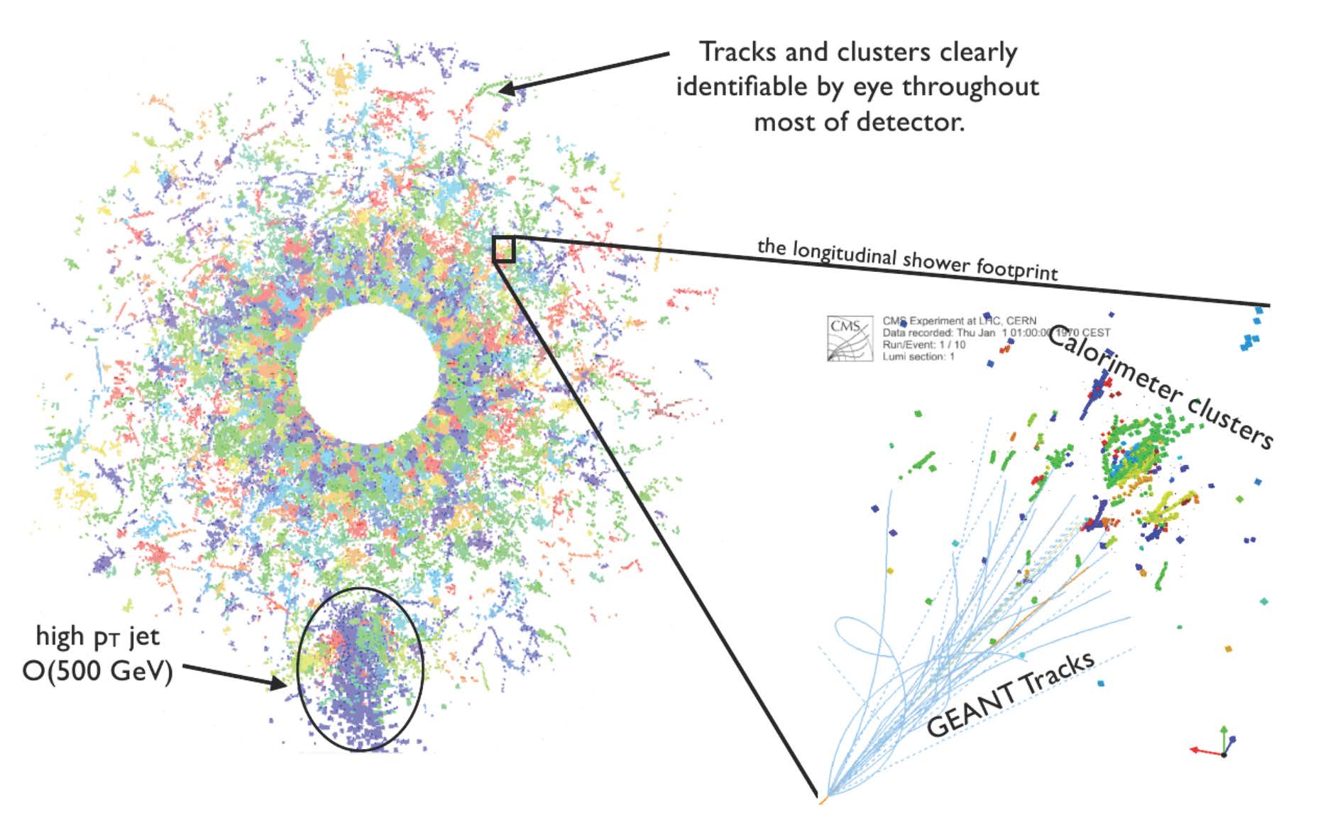
 High-energy physics research aims to understand the mysteries of the universe by describing the fundamental constituents of matter and the interactions between them. Diverse experiments exist on Earth to re-create the first instants of the universe. Two examples of the most complex experiments in the world are at the Large Hadron Collider (LHC) at CERN …
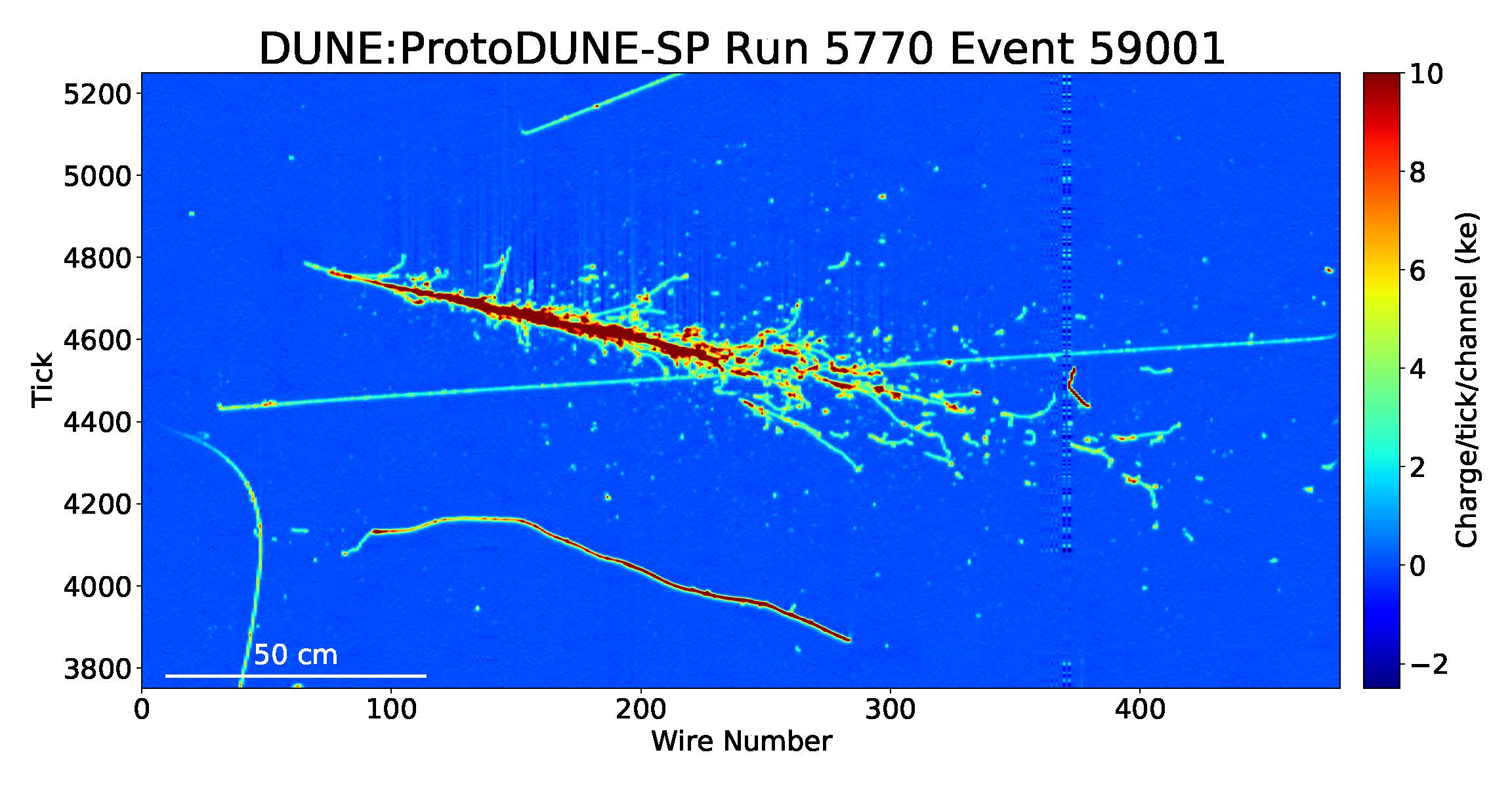
 Switzerland-based Assaia International AG is deploying a deep learning solution at Cincinnati/Northern Kentucky International Airport (CVG) to help airport employees monitor the turnaround time between flights.
  Today, NVIDIA is announcing the availability of nvCOMP version 2.0.0. This software can be downloaded now free for members of the NVIDIA Developer Program.
 Recommender systems drive engagement on many of the most popular online platforms. As data volume grows exponentially, data scientists increasingly turn from traditional machine learning methods to highly expressive, deep learning models to improve recommendation quality. Often, the recommendations are framed as modeling the completion of a user-item matrix, in which the user-item entry is …
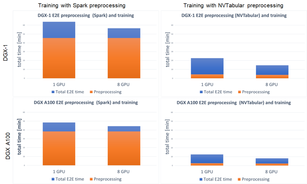

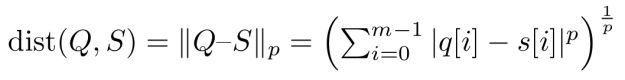
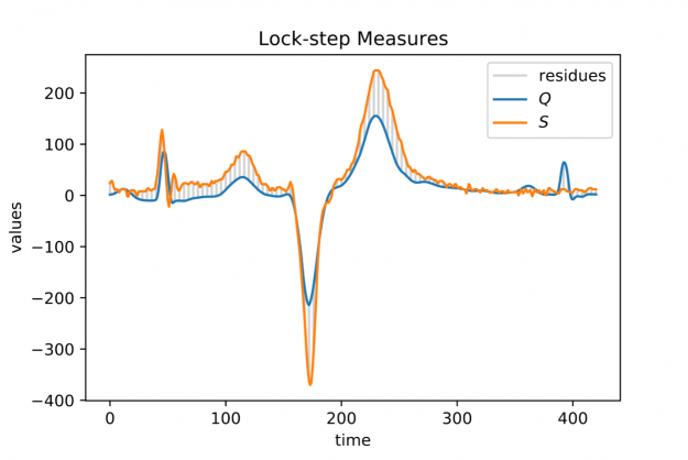
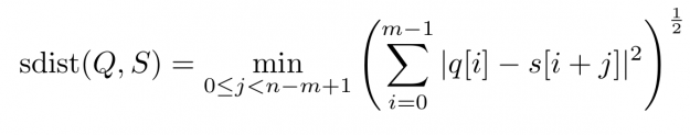
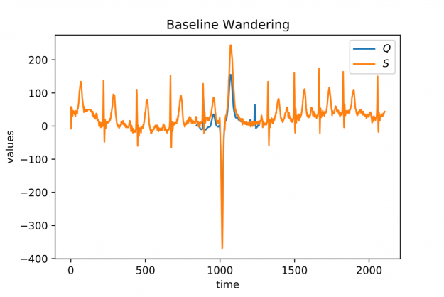
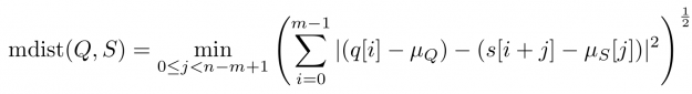
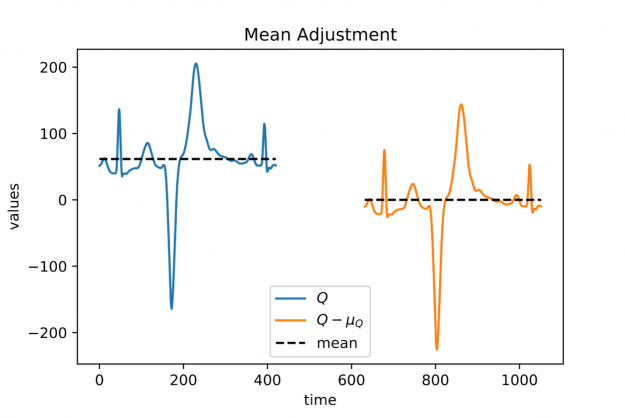
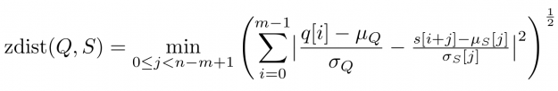
 To say it with the words of Eamonn Keogh: “Time series is a ubiquitous and increasingly prevalent type of data […]”. Virtually any incrementally measured signal, be it along a time axis or a linearly ordered set, can be treated as time series. Examples include electrocardiograms, temperature or voltage measurements, audio, server logs, but also …