
Categories
Category: Offsites
Stuff I find valuable at key websites
Categories
Sphere Intersection Puzzle Corrected
Categories
The Phone Number puzzle
Categories
The last IMO problem AI could not solve
Categories
The last IMO problem AI could not solve
Helios: hyperscale indexing for the cloud & edge, Potharaju et al., PVLDB’20
On the surface this is a paper about fast data ingestion from high-volume streams, with indexing to support efficient querying. As a production system within Microsoft capturing around a quadrillion events and indexing 16 trillion search keys per day it would be interesting in its own right, but there’s a lot more to it than that. Helios also serves as a reference architecture for how Microsoft envisions its next generation of distributed big-data processing systems being built. These two narratives of reference architecture and ingestion/indexing system are interwoven throughout the paper. I’m going to tackle the paper in two parts, focusing today on the reference architecture, and in the next post on the details of Helios itself. What follows is a discussion of where big data systems might be heading, heavily inspired by the remarks in this paper, but with several of my own thoughts mixed in. If there’s something you disagree with, blame me first!
Why do we need a new reference architecture?
Cloud-native systems represent by far the largest, most distributed, computing systems in our history. And the established cloud-native architectural principles behind them aren’t changing here. But zoom out one level of abstraction, and you can also look at cloud platforms as the largest, most-centralised, computing systems in our history. We push as much data processing as possible onto warehouse-scale computers and systems software. It’s a planet-scale client-server architecture with an enormous number of mostly thin clients sharing the services of a few giant server systems. There are several pressures on such a design:
- The volume of data continues to grow – by another 2 orders of magnitude this decade according to IDC – as does the velocity of data arrival and the variance in arrival rates. At the same time, end users want results faster – from batch to real-time.
We are observing significant demand from users in terms of avoiding batch telemetry pipelines altogether.
- It makes heavy use of comparatively expensive data-center computing facilities
- It’s limited by the laws of physics in terms of end-to-end latency
- It’s more challenging to build privacy-respecting systems when all data needs to shipped remotely to be processed
The first two of these pressures combine to cause cloud systems to run into one of two limits as exemplified by this quote from the paper:
None of our existing systems could handle these requirements adequately; either the solution did not scale or it was too expensive to capture all the desired telemetry. (Emphasis mine)
Latency limits are one of the drivers pushing us towards more edge computing – a trend which began with static content distribution, then dynamic content (both of which sit on the response path), and now is extending to true edge computation (that can also help improve the request path, e.g. by local processing either eliminating or reducing the amount of data that needs to be sent on to central servers). Industrial IoT use cases are an example here.
The emergence of edge computing has raised new challenges for big data systems… In recent years a number of distributed streaming systems have been built via either open source or industry effort (e.g. Storm, Spark Streaming, MillWheel, Dataflow, Quill). These systems however adopt a cloud-based, centralised architecture that does not include any “edge computing” component – they typically assum an external, independent data ingestion pipeline that directs edge streams to cloud storage endpoints such as Kafka or Event Hubs.
On the privacy front, with increasing awareness and regulation (a good thing, imho!), it’s getting much more complex and expensive to process, store, and secure potentially sensitive data. The most cost-effective mechanism of all is not to store it centrally, and not to process it centrally. Securing data you don’t have and never saw is free! In this regard the machine learning community is ahead of the systems community, with a growing body of work on federated machine learning.
The GDPR directive requires that companies holding EU citizen data provide a reasonable level of protection for personal data… including erasing all personal data upon request… Finding the list of data streams that contain the user’s information requires a provenance graph (as the number of streams is in the order of 10s of billions) and an index (as each stream can span multiple peta-bytes) to avoid expensive linear scans.
What does the new reference architecture look like?
The central idea in the Helios architecture is ’embrace the edge’. Although the word federated doesn’t actually appear in the paper at all, federated big-data systems (c.f. federated machine learning and federated database management systems) seems a reasonable way of describing what’s going on here.
Helios is an effort towards building a new genre of big data systems that combine the cloud and edge as a single, holistic data processing platform.
(And by extension, we could envision end-user devices being part of that holistic platform too).
In the olden days we used to talk about function shipping and data shipping. Function shipping being the idea that you move the compute to the data, and data shipping being the idea that you move the data to the compute. Within todays cloud systems, a lot of function shipping takes place, but for the clients that interact with them, it’s very heavily skewed towards data shipping. In federated big-data systems perhaps the appropriate terms would be function spreading and data spreading. I.e. compute can take place at multiple different points along the path from end device to cloud (and back again), and data can be spread out across layers too. A good guiding principle for designing such a system is probably to minimise data movement – i.e. (1) do as much processing as possible as close to the point of data capture as possible, and only send the aggregated results downstream, and then (2) where pools of data do amass, do as much querying of that data as close to the point of data storage as possible and only send the query results back upstream.
In Helios, this translates to coming up with efficient techniques for splitting computation between end devices, edge, and cloud.
This split has another interesting consequence. We saw earlier that there is end-user pressure to replace batch systems with much lower latency online systems. I observe that computation split across end devices, edge, and cloud doesn’t really sit well with batch processing either. We do distributed batch processing within a layer (e.g. map-reduce) but across layers is different. My conclusion is that federated big-data systems are also online systems. One nice advantage of unifying batch and online processing is that we don’t need to duplicate logic:
This solves the problem of maintaining code that needs to produce the same result in two complex distributed systems.
Generally batch systems have higher throughput and higher latency, and as we reduce the batch size towards online systems, we lower the latency and also the throughput. It will be interesting to watch the throughput characteristics of federated big data systems, but it’s a challenge I think we have to take on. (Helios’ throughput is plenty good enough btw.)
Technically, what might it look like to build a system that works in this way?
Based on our production experience, we posit that a single engine model can (1) enable optimizations such as automatically converting recurring batch queries into streaming queries, dynamically mapping operators/computations to various layers (e.g., end device, edge, cloud), automated A/B testing for figuring out the best query execution plans, join query optimization in multi-tenant scenarios and automatic cost-based view materialisation, and (2) significantly reduce user and operational burden of having to learn and maintain multiple complex stacks.
I’m going to throw one more requirement into the mix for next-generation big data systems. You won’t find this in the Helios paper, but it is something that Microsoft have articulated well in other works, notably Cloudy with a high chance of DBMS: a 10-year prediction for enterprise-grade ML . From a data systems perspective, machine learning is just data processing over (usually) big data sets. We don’t really want completely separate systems for federated machine learning and federated big-data, especially as there are many data cycles between the two (ML both consuming and producing data) and ML is increasingly becoming a mainstream part of many systems and applications. See e.g. the introduction to ‘The case for a learned sorting algorithm.’
The picture that forms in my mind is of a federated differential dataflow style system that processes and materializes just what is needed at each layer. E.g. in the Helios case, “we can similarly distribute the task of data summarization – including filtering, projections, index generation, and online aggregation – to end devices.” One nice thing that falls out of extending such a system all the way out to the end devices is that it means the dataflow engine is effectively responsible for managing all of those pesky caches, and especially cache invalidation.
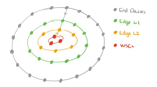
There might be many different layers of edge compute (e.g. 5G base stations, CDN POPs, …) between an end-(user) device and a warehouse scale computer (WSC, aka the cloud). You can think of these as concentric rings forming around WSCs, and conceptually a federated big data system can span all of them.
So far we’ve mostly been talking about spreading compute and data along a single path from an end device to the cloud and back again, leading to a picture like this.
But of course it’s entirely possible (and common) for a node at one layer to interact with multiple nodes at the layer below, leading to a picture more like this:

And furthermore it’s easy to imagine cases where peer-to-peer communication between nodes at the same level also makes sense:

In general we’re looking at a dynamic dataflow topology with very large numbers of nodes.
Helios is a successful production example of a subset of these ideas, and we’ll look at Helios itself in much more detail in the next post. For now I’ll close with this thought:
Helios provides one example for a specific type of computation, i.e. indexing of data. There are a number of related problems, such as resource allocation, query optimization, consistency, and fault tolerance. We believe that this is a fertile ground for future research.
Categories
The case for a learned sorting algorithm
The case for a learned sorting algorithm, Kristo, Vaidya, et al., SIGMOD’20
We’ve watched machine learning thoroughly pervade the web giants, make serious headway in large consumer companies, and begin its push into the traditional enterprise. ML, then, is rapidly becoming an integral part of how we build applications of all shapes and sizes. But what about systems software? It’s earlier days there, but ‘The case for learned index structures’(Part 1 Part 2), SageDB and others are showing the way.
Today’s paper choice builds on the work done in SageDB, and focuses on a classic computer science problem: sorting. On a 1 billion item dataset, Learned Sort outperforms the next best competitor, RadixSort, by a factor of 1.49x. What really blew me away, is that this result includes the time taken to train the model used!
The big idea
Suppose you had a model that given a data item from a list, could predict its position in a sorted version of that list. 0.239806? That’s going to be at position 287! If the model had 100% accuracy, it would give us a completed sort just by running over the dataset and putting each item in its predicted position. There’s a problem though. A model with 100% accuracy would essentially have to see every item in the full dataset and memorise its position – there’s no way training and then using such a model can be faster than just sorting, as sorting is a part of its training! But maybe we can sample a subset of the data and get a model that is a useful approximation, by learning an approximation to the CDF (cumulative distribution function).
If we can build a useful enough version of such a model quickly (we can, we’ll discuss how later), then we can make a fast sort by first scanning the list and putting each item into its approximate position using the model’s predictions, and then using a sorting algorithm that works well with nearly-sorted arrays (Insertion Sort) to turn the almost-sorted list into a fully sorted list. This is the essence of Learned Sort.
A first try
The base version of Learned Sort is an out-of-place sort, meaning that it copies the sorted elements into a new destination array. It uses the model to predict the slot in the destination array for each item in the list. What should happen though if the model predicts (for example) slot 287, but there’s already an entry in the destination array in that slot? This is a collision. The candidate solutions are:
- Linear probing: scan the array for nearest vacant slot and put the element there
- Chaining: use a list or chain of elements for each position
- A Spill bucket: if the destination slot is already full, just put the item into a special spill bucket. At the end of the pass, sort and merge the spill bucket with the destination array.
The authors experimented with all three, and found that the spill bucket approach worked best for them.

The resulting performance depends on the quality of the model predictions, a higher quality model leads to fewer collisions, and fewer out-of-order items to be patched in the final Insertion Sort pass. Since we’re punting on the details of the model for the moment, an interesting question is what happens when you give this learned sort a perfect, zero-overhead oracle as the model? Say we want to sort all the numbers from zero to one billion. A perfect zero-overhead oracle can be built by just using the item value as the position prediction. 1456? That will go in position 1456…
And what did happen when the authors tried to sort the numbers using this perfect zero-overhead oracle?
To our astonishment, in this micro-experiment we observed that the time take to distributed the keys into their final sorted position, despite a zero-overhead oracle function, took 38.7 sec and RadixSort took 37.5 sec.
Why? If it’s high performance you’re after, you can’t ignore mechanical sympathy. Radix Sort is carefully designed to make effective use of the L2 cache and sequential memory accesses, whereas Learned Sort is making random accesses all over the destination array.
Sympathy for the machine
How can learned sort be adapted to make it cache-efficient? The solution is to change the first pass of Learned Sort into a cascading Bucket Sort. Instead of determining the final position in the destination array, the model prediction is used to ascertain which bucket (or bin) the element should go into.
- Let
be the number of buckets (
is reached. If at any stage a model prediction places in an item in a bucket that is already full, this item is just moved to a spill bucket instead.
- Once we’re down to buckets of size
- Concatenate the sorted buckets in order (some may have less than elements in them), and use Insertion Sort to patch up any discrepancies in ordering.
- Sort and merge the spill bucket.
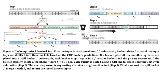
The secret to good performance with Learned Sort is choosing
The parameter
With these changes in place, if the number of elements to sort is close to the key domain size (e.g. sorting 2^32 elements with 32-bit keys), then Learned Sort performs almost identically to Radix Sort. But when the number of elements is much smaller than the key domain size, Learned Sort can significantly outperform Radix Sort.
Oh, yes – about the model!
All of this depends of course on being able to train a sufficiently accurate model that can make sufficiently fast predictions, so that the total runtime for Learned Sort, including the training time still beats Radix Sort. For this, the authors use the Recursive Model Index (RMI) architecture as first introduced in ‘The case for learned index structures‘. In brief, RMI uses layers of simple linear models arranged in a hierarchy a bit like a mixture of experts.
During inference, each layer of the model takes the key as an input and linearly transforms it to obtain a value, which is used as an index to pick a model in the next layer.
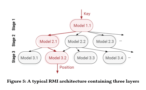
The main innovation the authors introduce here is the use of linear spline fitting for training (as opposed to e.g. linear regression with an MSE loss function). Spline fitting is cheaper to compute and gives better monotonicity (reducing the time spent in the Insertion Sort phase). Each individual spline model fits worse than its closed-form linear regression counterpart, but the hierarchy compensates. Linear splines result in 2.7x faster training, and up to 35% fewer key swaps during Insertion Sort.
Evaluation
On synthetic datasets containing double-precision keys following a standard normal distribution, the authors compared Learned Sort to a variety of cache-optimized and highly tuned C++ implementations of alternative sorting algorithms, presenting the most competitive alternatives in their results. The following chart shows sorting rates over input dataset sizes varying from one million to one billion items.
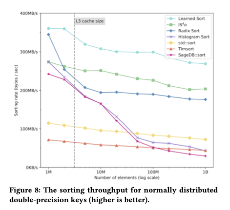
Learned Sort outperforms the alternative at all sizes, but the advantage is most significant when the data no longer fits into the L3 cache – an average of 30% higher throughput than the next best algorithm.
The results show that our approach yields an average 3.38x performance improvement over C++ STL sort, which is an optimized Quick- sort hybrid, 1.49x improvement over sequential Radix Sort, and 5.54x improvement over a C++ implementation of Tim- sort, which is the default sorting function for Java and Python.
Learned Sort’s advantage holds over real datasets as well (§6.1 for datasets included in the test), and for different element types:
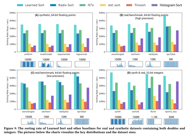
[Learned Sort] results in significant performance improvements as compared to the most competitive and widely used sorting algorithms, and marks an important step into building ML-enhanced algorithms and data structures.
Extensions
The paper also describes several extensions to Learned Sort including sorting in-place, sorting on other key types (strings initially), and improving performance for datasets with many duplicate items.
Categories
Bias in word embeddings
Bias in word embeddings, Papakyriakopoulos et al., FAT*’20
There are no (stochastic) parrots in this paper, but it does examine bias in word embeddings, and how that bias carries forward into models that are trained using them. There are definitely some dangers to be aware of here, but also some cause for hope as we also see that bias can be detected, measured, and mitigated.
…we want to provide a complete overview of bias in word embeddings: its detection in the embeddings, its diffusion in algorithms using the embeddings, and its mitigation at the embeddings level and at the level of the algorithm that uses them.
It’s been shown before (‘Man is to computer programmer as woman is to homemaker?’) that word embeddings contain bias. The dominant source of that bias is the input dataset itself, i.e. the text corpus that the embeddings are trained on. Bias in, bias out. David Hume put his finger on the fundamental issue at stake here back in 1737 when he wrote about the unjustified shift in stance from describing what is and is not to all of a sudden talking about what ought or ought not to be. The inputs to a machine learning model are a description of what is. If we train a model on them within thinking, the outputs of the model will treat what is as if it were what ought to be. We have made a sophisticated machine for reinforcing the status quo, warts and all.
When it comes to word embeddings this effect can be especially powerful because the embeddings isolate the words from the contexts in which they were originally used, leaving behind a static residue of bias:
…the projection of words in a mathematical space by the embeddings consolidates stereotyping and prejudice, assigning static properties to social groups and individuals. Relations are no longer context-dependent and dynamic, and embeddings become deterministic projections of the bias of the social world. This bias is diffused into further algorithms unchanged, resulting in socially discriminative decisions.
The authors proceed in the following manner:
- Firstly, they train one set of word embeddings based on the complete German wikipedia, and another set based on Facebook and Twitter content relating to the six main political parties in Germany. The training is done using GloVe. To be able to compare these word embeddings (by placing them both within the same vector space), they then find the linear transformation matrix that places all words from one into the vector space of the other with minimal translation. Since the translation is linear, the normalised distance between words does not change and hence any bias is preserved.
- They then measure bias in the trained embeddings
- Having demonstrated that the word embeddings do indeed contain bias, the next step is to see if a model trained using these word embeddings exhibits bias in its outputs (which they show it does).
- Given the resulting models does show bias, they then explore mechanisms for mitigating that bias at both the word embedding level and at the level of the final trained classifier.
- Finally, they show how biased word embeddings can actually help us to detect the same biases in new text samples (for example, the output of a language model?).
Measuring bias in word embeddings
Say we want to know whether a word embedding for a concept has a gender bias. We can take the cosine distance between and ‘Man’ and subtract the cosine distance between and ‘Woman’. A non-zero result reveals bias in one direction or the other, and the magnitude of the result tells us the amount of the bias. Since the study is done using the German language, which is gendered, concepts with male and female versions are represented by word pairs. This basic technique is used to assess bias in the trained word embeddings for professions, for Germans vs foreigners, and for homosexual vs heterosexual.
The results show that the trained vectors are more likely to associated women with professions such as nursing and secretarial work, whereas men are associated with roles such as policemen and commanders. Germans are linked to positive sentiments such as charm and passion, cooperation and union, while foreigners are generally linked to concepts such as immigration, law, and crime. Homosexuals are related to roles such as hairdresser or artist, and heterosexuals to blue collar professions and science. Homosexuality was associated with negative sentiments, and heterosexuality with positive ones.
Summaries of the most extremely biased words in both the Wikipedia and social media data sets are given in the tables below.
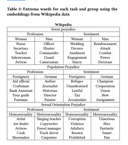
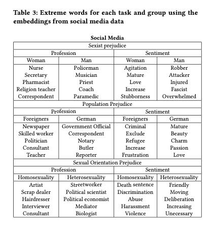
[the] results illustrate that word embeddings contain a high level of bias in them in terms of group stereotypes and prejudice. The intergroup comparison between sexes, populations, and sexual orientations revealed the existence of strong stereotypes and unbalanced evaluation of groups. Although Wikipedia contained a stronger bias in terms of stereotypes, social media contained a higher bias in terms of group prejudice.
Do biased word embeddings lead to biased models?
The authors trained a model that took a word embedding as input and predicted whether that word has a positive or negative sentiment. To assess bias in the trained model, the authors fed names as inputs with the expectation that in the absence of bias, names should have a zero sentiment score as they are polarity independent. The chosen names were stereotypical first names for nine population groups: German, Turkish, Polish, Italian, Greek, French, US American, Russian, and Arabic. The authors also compared male and female names.
The study illustrated the use of biased word embeddings results in the creation of biased machine learning classifiers. Models trained on the embeddings replicate the preexisting bias. Bias diffusion was proved both for sexism and xenophobia, with sentiment classifiers assigning positive sentiments to Germans and negative sentiments to foreigners. In addition, the amount of polarity for men and women in the embeddings was diffused unaltered into the models.
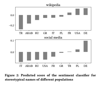
Mitigating bias
The authors investigate two different methods for bias mitigation in the sentiment classifier:
- Removing bias at the individual word embedding level (by making theoretically neutral words orthogonal to the sentiment vector, where the sentiment vector is e.g. good – bad, positive – negative etc.).
- Removing bias at the level of the classifier by adjusting the linear hyperplane learned by the linear SVM classifier, such that this plane is orthogonal to the sentiment vector.
While both methods reduce bias in the resulting classifications, the classifier-level correction is much more effective, as can be seen in the following figure.
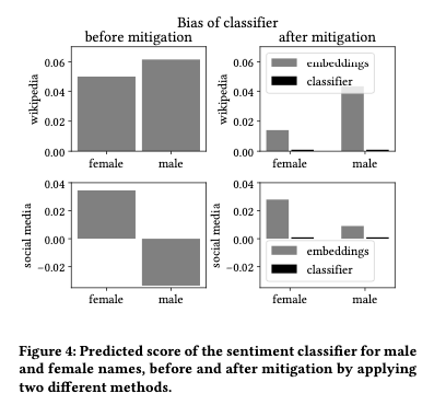
This is because correcting embeddings for a theoretically neutral set of words still leaves other potential biases in place that weren’t corrected for. The classifier is good at finding these!
…the classifier learns further associations between the vectors, which are not taken into consideration when debiasing at the embeddings level… Hence, we show that debiasing at the classifier level is a much better and safer methodology to follow.
Detecting bias in text
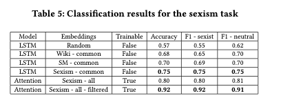
The authors created a dataset containing an equal number of sexist and non-sexist comments from Facebook pages of German political parties. Then they trained models with LSTM and attention-based architectures to classify comments as sexist or non-sexist. Multiple variants were trained, using random embeddings, the Wikipedia embeddings, the social media embeddings, and embeddings trained on the sexist comments.
The more similar the bias in the embeddings with the target data, the higher the ability of the classifier to detect them.
The attention-based network architecture, when given the sexism embeddings, allowed to freely retrain them, and tested on comments only containing words with embeddings, achieved an accuracy of 92%.
A call to action
The study showed that bias in word embeddings can result in algorithmic social discrimination, yielding negative inferences on specific social groups and individuals. Therefore, it is necessary not only to reflect on the related issues, but also to develop frameworks of action for the just use of word embeddings…
When it comes to generative language models, one possibility that strikes me is to use the model to generate a text corpus, train word embeddings on that corpus, and then analyse them for bias. Any detected bias could then be fed back into the language model training process as a form of negative reinforcement.