 Discover the latest traditional and neural rendering technologies and how they are accelerating professional visualization.
Discover the latest traditional and neural rendering technologies and how they are accelerating professional visualization.
 DataBloom
Discover the latest traditional and neural rendering technologies and how they are accelerating professional visualization.
Discover the latest traditional and neural rendering technologies and how they are accelerating professional visualization.
 In computer graphics, the right balance between direct and indirect lighting elevates the photorealism of a scene.
In computer graphics, the right balance between direct and indirect lighting elevates the photorealism of a scene.
") Recommendation systems are widely used today to personalize user experiences and improve customer engagement in various settings like e-commerce, social media,…
Recommendation systems are widely used today to personalize user experiences and improve customer engagement in various settings like e-commerce, social media,…
Recommendation systems are widely used today to personalize user experiences and improve customer engagement in various settings like e-commerce, social media, and news feeds. Serving user requests with low latency and high accuracy is hence critical to sustain user engagement.
This includes performing high-speed lookups and computations while seamlessly refreshing models with the newest updates, which is especially challenging for large-scale recommenders where the model size exceeds GPU memory.
NVIDIA Merlin HugeCTR, an open-source framework designed to optimize large-scale recommenders on NVIDIA GPUs, recently released Hierarchical Parameter Server (HPS) architecture to specifically address the needs of industry-grade inference systems. Experiments indicate that this approach enables scalable deployment with low latency on popular benchmarking datasets.
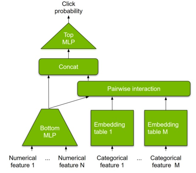
Large embedding tables: The inputs to typical deep recommendation models can be numerical (user age or item price, for example) or categorical features (user ID or item ID, for example). Unlike numerical features, categorical features need to be transformed into numerical vectors to be fed into multilayer perceptron (MLP) layers for dense computation. This is facilitated by an embedding table that learns a mapping (“embeddings”) from the categorical to the numerical feature space.
Embedding tables are therefore part of the model parameters and can be memory-intensive, reaching up to TB-scale for modern recommender systems. This is well beyond the onboard memory capacity of modern GPUs. Consequently, most existing solutions fall back to hosting embedding tables in CPU memory, which does not take advantage of high-bandwidth GPU memory leading to higher end-to-end latencies.
Scalability: Driven by user behavior, many customer applications are built to serve peak usages, and need the flexibility to scale-out or scale-up the AI inference engine based on their expected and actual load.
Framework and platform agnostic: The AI inference engine must be able to serve both deep-learning models (DeepFM, DCN, DLRM, MMOE, DIN, and DIEN, for example) trained by frameworks like TensorFlow or PyTorch, as well as simple machine learning (ML) models. In addition, customers desire hybrid deployment of both multiple different model architectures and multiple instances of a single model. Models must also be deployed across a variety of hardware platforms from cloud to edge.
Deploying new models and online training updates: Customers want the option to frequently update their models according to market trends and new user data. Model updates should be seamlessly applied to inference deployments.
Fault tolerance and high availability: Customers need to maintain the same level of SLA, preferably five-nines or above for mission-critical applications.
The following section provides more details about how NVIDIA Merlin HugeCTR addresses these challenges using HPS to enable large-scale inference for recommendations.
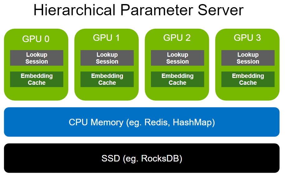
The Hierarchical Parameter Server enables deployment of large recommendation inference workloads using a multi-level adaptive storage solution. To store large-scale embeddings, it uses GPU memory as the first-level cache, CPU memory as second-level cache (such as HashMap for local deployment and Redis for distributed), and SSD for extended storage capacity (such as RocksDB).
Both CPU memory and SSD can be flexibly configured based on the user’s needs. Note that the size of dense layers (MLPs) is much smaller in comparison to embeddings. Therefore, dense layers are replicated across the various GPU workers in a data-parallel fashion.
The memory bandwidth of GPUs is an order of magnitude higher than that of most CPUs. For example, NVIDIA A100-80 GB provides more than 2 TB/s HBM2 bandwidth. The GPU embedding cache leverages such high memory bandwidth by moving the memory-intensive embedding lookups into the GPU, closer to where the compute happens.
To design a system that efficiently leverages the advantages offered by modern GPUs, it is important to take note of one key observation: with real-world recommendation datasets, a few feature categories typically occur much more frequently than others. For example, in the Criteo 1 TB Click Logs dataset, a popular benchmarking dataset also used in MLPerf, 305K categories out of a total 188M (representing just 0.16%) are referenced by 95.9% of all samples.
This implies that some embeddings are accessed far more frequently than others. Embedding key accesses roughly follow a power-law distribution. Consequently, caching these most frequently accessed parameters in GPU memory will enable recommender systems to take advantage of high GPU memory bandwidth. Individual embedding lookups are independent, which makes GPUs the ideal platform for vector lookup processing, with their ability to run thousands of threads concurrently.
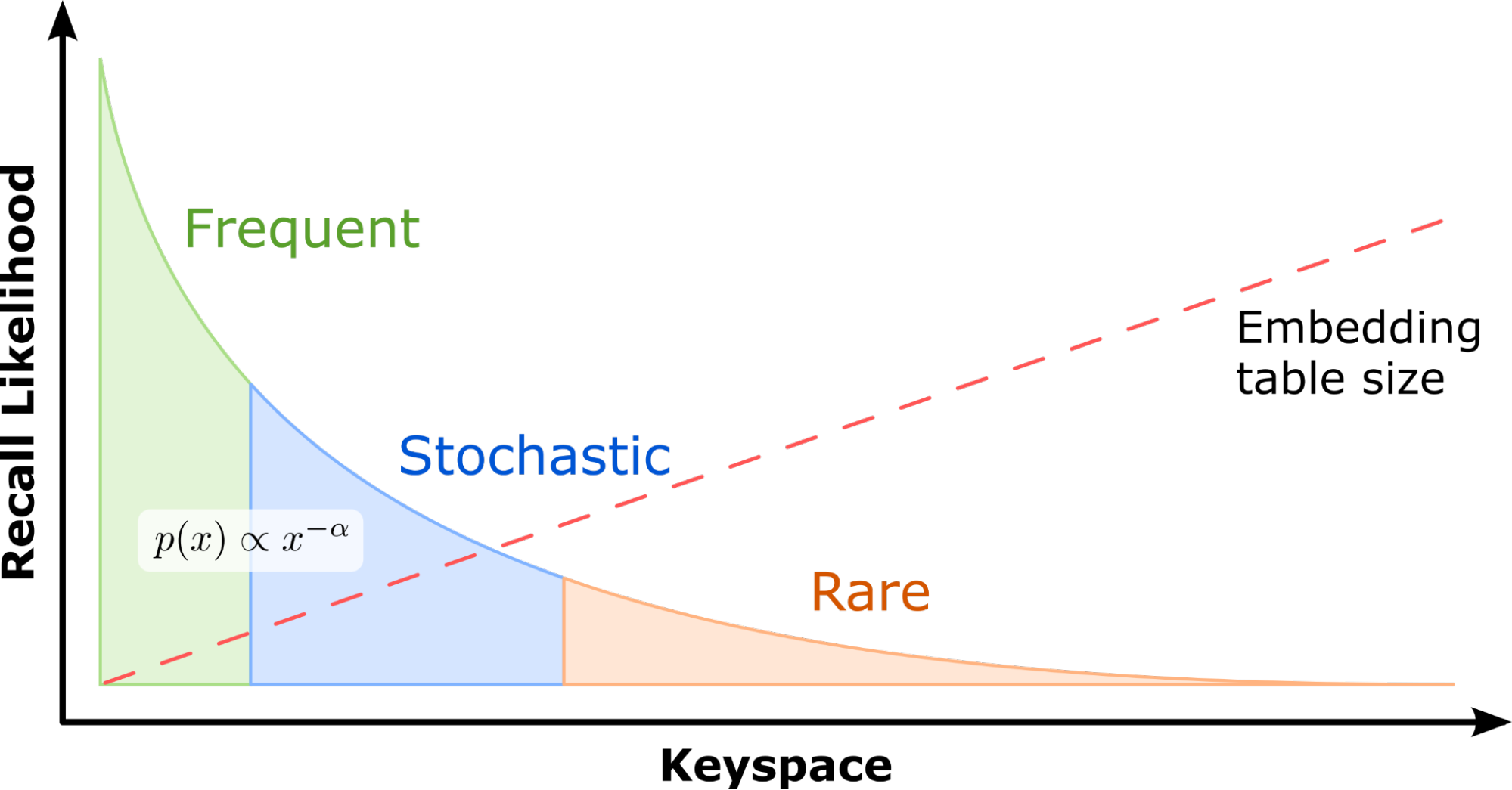
These properties have inspired the design of the HPS GPU embedding cache that retains the hot embeddings in GPU memory, improving lookup performance by reducing additional or repetitive parameter movement across a slower CPU-GPU bus. It is backed by secondary storage that keeps a full copy of all the embedding tables. This is explored more fully below. A unique GPU embedding cache exists for each embedding table associated with each model hosted on a GPU.
When looked-up embedding keys are missing in the GPU cache during inference, a key insertion is triggered to fetch the related data from lower levels of the hierarchy. The HPS implements both synchronous and asynchronous key insertion mechanisms, and a user-defined hit rate threshold to choose between the two options to balance accuracy and latency.
Figure 4, shows the measured inference latency versus hit rate with the Criteo 1 TB Click Logs dataset and the 90 GB Deep Learning Recommendation Model for Personalization and Recommendation Systems (DLRM) model on an NVIDIA T4 (16 GB memory), A30 (24 GB memory) and A100 GPU (80 GB memory), caching 10% of the model size. The hit rate threshold is set to 1.0, so that all key insertions are synchronous. Measurements are taken at the stable stage.
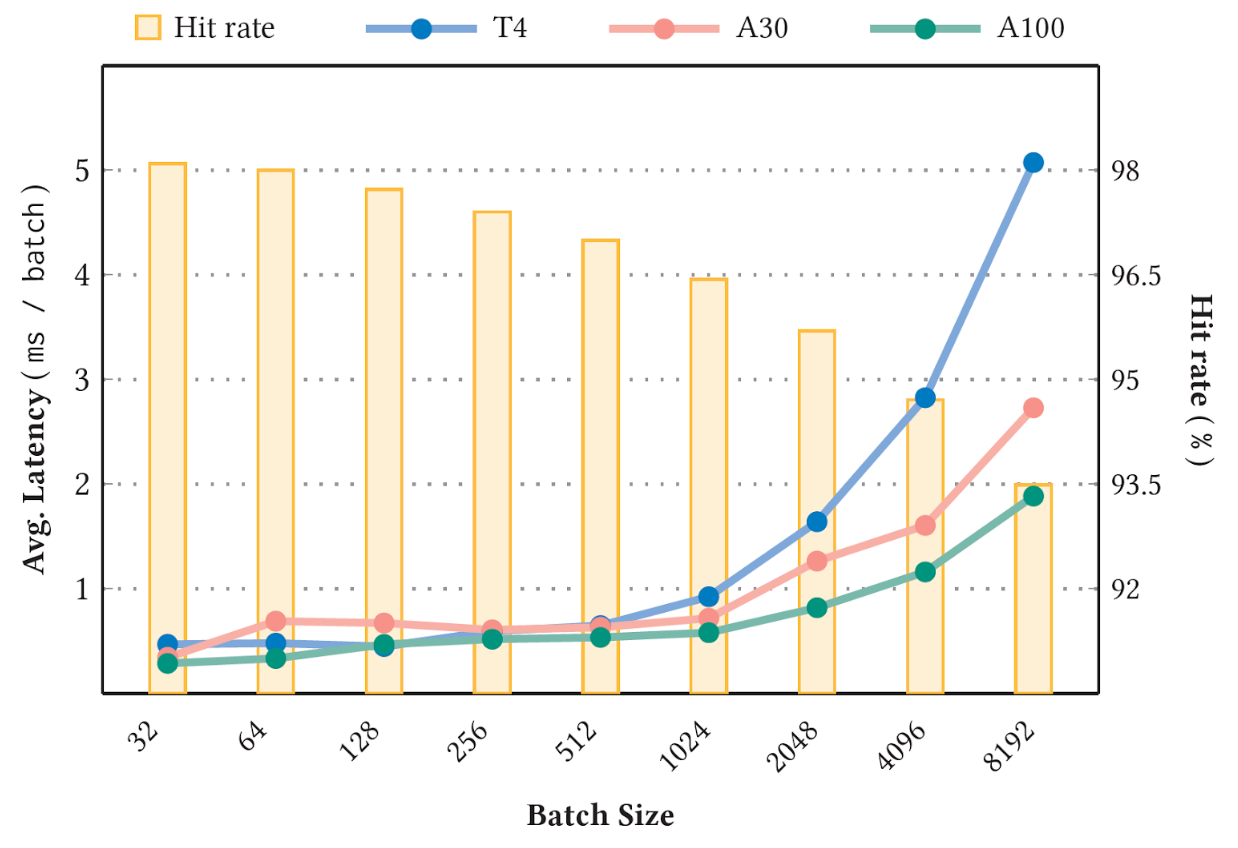
As can be expected, a higher stable cache hit rate (the bar chart in Figure 4) corresponds to a lower average latency (the line chart in Figure 4). Moreover, a larger batch size also witnesses lower hit rate and higher latency due to the increasing likelihood of keys missing. For more details about the benchmark, see A GPU-Specialized Inference Parameter Server for Large-Scale Deep Recommendation Models.
HPS includes two additional layers to support models that scale beyond GPU memory capacity by leveraging the CPU memory and SSD. These layers are highly configurable to support various backend implementations. The following sections take a closer look at these.
The second-level storage is the CPU cache, accessed through the CPU-GPU bus, and acts as the extended storage for the GPU embedding cache at lower cost. If an embedding key is missing in the GPU embedding cache, HPS turns to querying the CPU cache next.
The ‘CPU cache’ layer supports various database backends. HugeCTR HPS provides volatile database examples with a hash map based local CPU memory database implementation, and a Redis cluster-based backend that leverages distributed cluster instances for scalable deployment.
The lowest level of the cache hierarchy stores an entire copy of each embedding table on either SSDs, hard disks, or a network storage volume at even lower cost. It is particularly effective with datasets that exhibit an extreme long-tail distribution (a very large number of categories, many of which are not referenced very often) where maintaining a high accuracy is critical for the task at hand. The HugeCTR HPS reference configuration maps embedding tables to column groups in a RocksDB database on a local SSD.
The entire model is persisted in each inference node by design. Such resource isolation strategies enhance system availability. The model parameters and inference service can be recovered even if just one node is alive after a catastrophic event.
Recommendation models have two modes of training: offline and online. Online training deploys fresh model updates into real-time production and is critical for recommendation effectiveness. HPS employs a seamless update mechanism through an Apache Kafka-based message buffers to connect training and inference nodes, as illustrated in Figure 5.
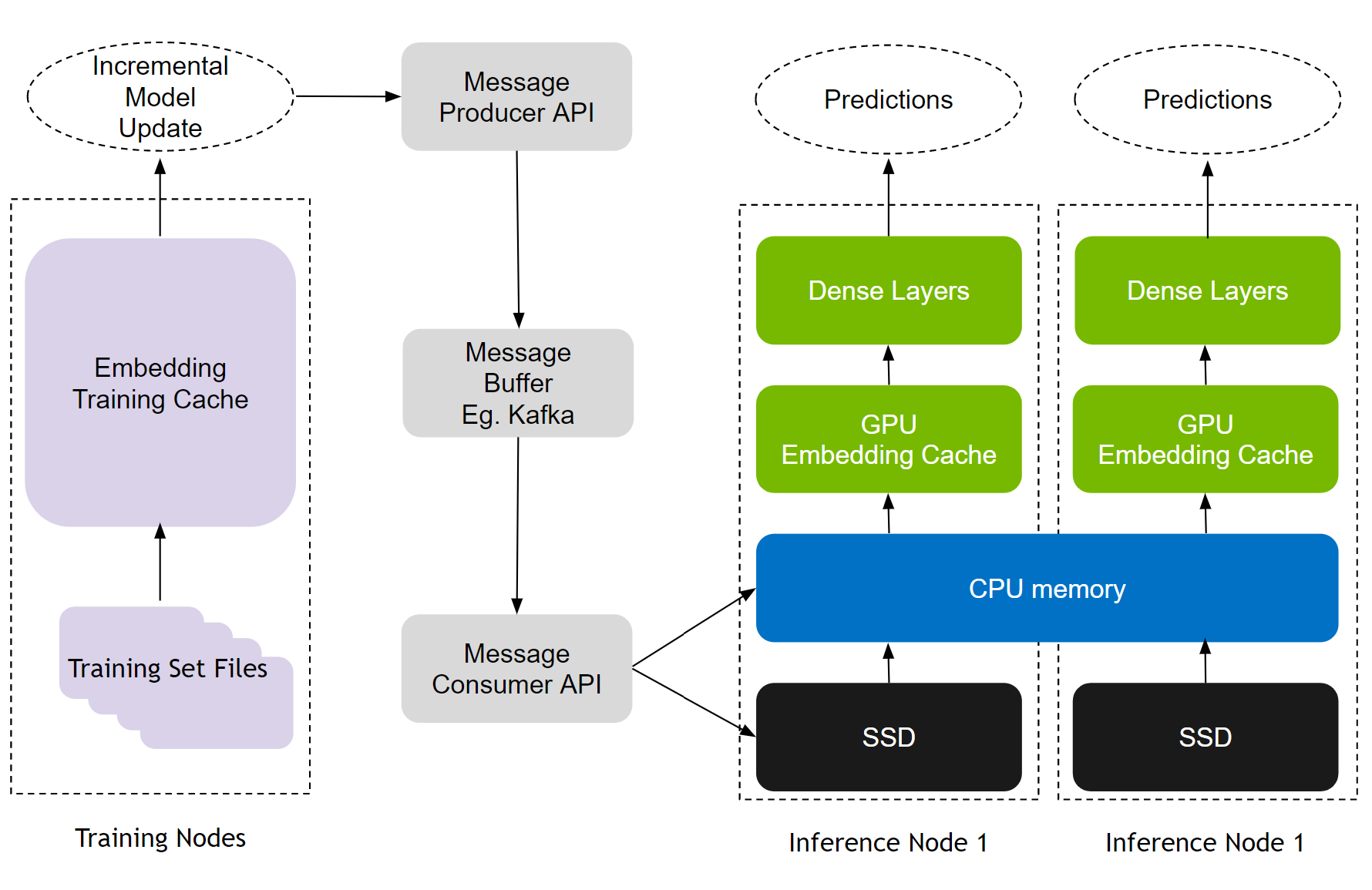
The update mechanism aids MLOps workflows, enabling both online/frequent as well as offline/retraining updates with no downtime. It also imparts fault tolerance by design, as training updates continue to queue up in the Kafka message buffer even if inference servers are down. All these capabilities are available to developers through convenient and easy-to-use Python APIs.
To demonstrate the benefits of HugeCTR HPS, we evaluated its end-to-end inference performance on the DLRM model and Criteo 1 TB Click Logs dataset, and compared it with scenarios where just the dense layer computations run on a GPU, and a CPU-only solution.
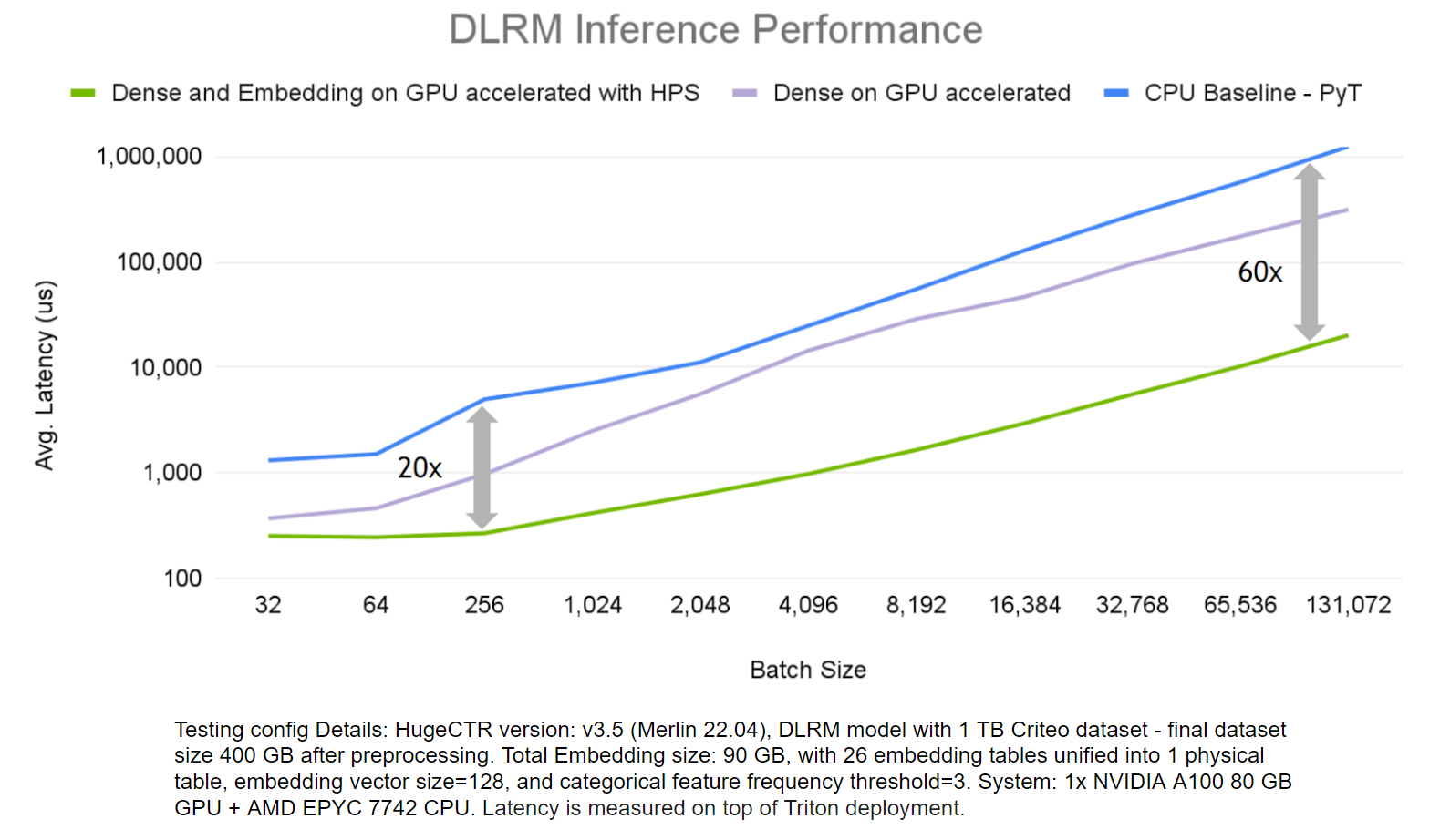
The HPS solution accelerates both embedding and dense layers far outperforms the CPU-only solution, up to 60x on larger batch sizes.
You may be familiar with CPU parameter server (PS) plus GPU worker solutions. Table 1 shows how the HPS differs from most PS plus worker solutions.
| HPS | CPU PS + GPU Worker | |
| Pipeline focus | Inference | Training and Inference |
| Embedding lookup GPU accelerated | Yes | No |
| GPU use | Most frequently accessed embedding tables Dense parameters from MLP |
Dense parameters from MLP |
| Inter GPU Communication | None | None |
| CPU use | Less frequently accessed embeddings | All embedding tables are sharded across CPUs |
This post presents the Merlin HugeCTR HPS with GPU embedding cache as a tool to accelerate inference with large-scale embeddings on NVIDIA GPUs. HPS is available through convenient and easy-to-use configurations, and includes examples to get you started. There will also be a TensorFlow plug-in coming that enables the use of HPS in an existing TF inference pipeline. For more details, see A GPU-Specialized Inference Parameter Server for Large-Scale Deep Recommendation Models and the Merlin HugeCTR HPS Documentation.
To learn more about best practices for building and deploying recommender systems on NVIDIA GPUs, see the Deep Learning Performance Documentation.
Patent documents typically use legal and highly technical language, with context-dependent terms that may have meanings quite different from colloquial usage and even between different documents. The process of using traditional patent search methods (e.g., keyword searching) to search through the corpus of over one hundred million patent documents can be tedious and result in many missed results due to the broad and non-standard language used. For example, a “soccer ball” may be described as a “spherical recreation device”, “inflatable sportsball” or “ball for ball game”. Additionally, the language used in some patent documents may obfuscate terms to their advantage, so more powerful natural language processing (NLP) and semantic similarity understanding can give everyone access to do a thorough search.
The patent domain (and more general technical literature like scientific publications) poses unique challenges for NLP modeling due to its use of legal and technical terms. While there are multiple commonly used general-purpose semantic textual similarity (STS) benchmark datasets (e.g., STS-B, SICK, MRPC, PIT), to the best of our knowledge, there are currently no datasets focused on technical concepts found in patents and scientific publications (the somewhat related BioASQ challenge contains a biomedical question answering task). Moreover, with the continuing growth in size of the patent corpus (millions of new patents are issued worldwide every year), there is a need to develop more useful NLP models for this domain.
Today, we announce the release of the Patent Phrase Similarity dataset, a new human-rated contextual phrase-to-phrase semantic matching dataset, and the accompanying paper, presented at the SIGIR PatentSemTech Workshop, which focuses on technical terms from patents. The Patent Phrase Similarity dataset contains ~50,000 rated phrase pairs, each with a Cooperative Patent Classification (CPC) class as context. In addition to similarity scores that are typically included in other benchmark datasets, we include granular rating classes similar to WordNet, such as synonym, antonym, hypernym, hyponym, holonym, meronym, and domain related. This dataset (distributed under the Creative Commons Attribution 4.0 International license) was used by Kaggle and USPTO as the benchmark dataset in the U.S. Patent Phrase to Phrase Matching competition to draw more attention to the performance of machine learning models on technical text. Initial results show that models fine-tuned on this new dataset perform substantially better than general pre-trained models without fine-tuning.
The Patent Phrase Similarity Dataset
To better train the next generation of state-of-the-art models, we created the Patent Phrase Similarity dataset, which includes many examples to address the following problems: (1) phrase disambiguation, (2) adversarial keyword matching, and (3) hard negative keywords (i.e., keywords that are unrelated but received a high score for similarity from other models ). Some keywords and phrases can have multiple meanings (e.g., the phrase “mouse” may refer to an animal or a computer input device), so we disambiguate the phrases by including CPC classes with each pair of phrases. Also, many NLP models (e.g., bag of words models) will not do well on data with phrases that have matching keywords but are otherwise unrelated (adversarial keywords, e.g., “container section” → “kitchen container”, “offset table” → “table fan”). The Patent Phrase Similarity dataset is designed to include many examples of matching keywords that are unrelated through adversarial keyword match, enabling NLP models to improve their performance.
Each entry in the Patent Phrase Similarity dataset contains two phrases, an anchor and target, a context CPC class, a rating class, and a similarity score. The dataset contains 48,548 entries with 973 unique anchors, split into training (75%), validation (5%), and test (20%) sets. When splitting the data, all of the entries with the same anchor are kept together in the same set. There are 106 different context CPC classes and all of them are represented in the training set.
| Anchor | Target | Context | Rating | Score |
| acid absorption | absorption of acid | B08 | exact | 1.0 |
| acid absorption | acid immersion | B08 | synonym | 0.75 |
| acid absorption | chemically soaked | B08 | domain related | 0.25 |
| acid absorption | acid reflux | B08 | not related | 0.0 |
| gasoline blend | petrol blend | C10 | synonym | 0.75 |
| gasoline blend | fuel blend | C10 | hypernym | 0.5 |
| gasoline blend | fruit blend | C10 | not related | 0.0 |
| faucet assembly | water tap | A22 | hyponym | 0.5 |
| faucet assembly | water supply | A22 | holonym | 0.25 |
| faucet assembly | school assembly | A22 | not related | 0.0 |
| A small sample of the dataset with anchor and target phrases, context CPC class (B08: Cleaning, C10: Petroleum, gas, fuel, lubricants, A22: Butchering, processing meat/poultry/fish), a rating class, and a similarity score. |
Generating the Dataset
To generate the Patent Phrase Similarity data, we first process the ~140 million patent documents in the Google Patent’s corpus and automatically extract important English phrases, which are typically noun phrases (e.g., “fastener”, “lifting assembly”) and functional phrases (e.g., “food processing”, “ink printing”). Next, we filter and keep phrases that appear in at least 100 patents and randomly sample around 1,000 of these filtered phrases, which we call anchor phrases. For each anchor phrase, we find all of the matching patents and all of the CPC classes for those patents. We then randomly sample up to four matching CPC classes, which become the context CPC classes for the specific anchor phrase.
We use two different methods for pre-generating target phrases: (1) partial matching and (2) a masked language model (MLM). For partial matching, we randomly select phrases from the entire corpus that partially match with the anchor phrase (e.g., “abatement” → “noise abatement”, “material formation” → “formation material”). For MLM, we select sentences from the patents that contain a given anchor phrase, mask them out, and use the Patent-BERT model to predict candidates for the masked portion of the text. Then, all of the phrases are cleaned up, which includes lowercasing and the removal of punctuation and certain stopwords (e.g., “and”, “or”, “said”), and sent to expert raters for review. Each phrase pair is rated independently by two raters skilled in the technology area. Each rater also generates new target phrases with different ratings. Specifically, they are asked to generate some low-similarity and unrelated targets that partially match with the original anchor and/or some high-similarity targets. Finally, the raters meet to discuss their ratings and come up with final ratings.
Dataset Evaluation
To evaluate its performance, the Patent Phrase Similarity dataset was used in the U.S. Patent Phrase to Phrase Matching Kaggle competition. The competition was very popular, drawing about 2,000 competitors from around the world. A variety of approaches were successfully used by the top scoring teams, including ensemble models of BERT variants and prompting (see the full discussion for more details). The table below shows the best results from the competition, as well as several off-the-shelf baselines from our paper. The Pearson correlation metric was used to measure the linear correlation between the predicted and true scores, which is a helpful metric to target for downstream models so they can distinguish between different similarity ratings.
The baselines in the paper can be considered zero-shot in the sense that they use off-the-shelf models without any further fine-tuning on the new dataset (we use these models to embed the anchor and target phrases separately and compute the cosine similarity between them). The Kaggle competition results demonstrate that by using our training data, one can achieve significant improvements compared with existing NLP models. We have also estimated human performance on this task by comparing a single rater’s scores to the combined score of both raters. The results indicate that this is not a particularly easy task, even for human experts.
| Model | Training | Pearson correlation |
| word2vec | Zero-shot | 0.44 |
| Patent-BERT | Zero-shot | 0.53 |
| Sentence-BERT | Zero-shot | 0.60 |
| Kaggle 1st place single | Fine-tuned | 0.87 |
| Kaggle 1st place ensemble | Fine-tuned | 0.88 |
| Human | 0.93 |
| Performance of popular models with no fine-tuning (zero-shot), models fine-tuned on the Patent Phrase Similarity dataset as part of the Kaggle competition, and single human performance. |
Conclusion and Future Work
We present the Patent Phrase Similarity dataset, which was used as the benchmark dataset in the U.S. Patent Phrase to Phrase Matching competition, and demonstrate that by using our training data, one can achieve significant improvements compared with existing NLP models.
Additional challenging machine learning benchmarks can be generated from the patent corpus, and patent data has made its way into many of today’s most-studied models. For example, the C4 text dataset used to train T5 contains many patent documents. The BigBird and LongT5 models also use patents via the BIGPATENT dataset. The availability, breadth and open usage terms of full text data (see Google Patents Public Datasets) makes patents a unique resource for the research community. Possibilities for future tasks include massively multi-label classification, summarization, information retrieval, image-text similarity, citation graph prediction, and translation. See the paper for more details.
Acknowledgements
This work was possible through a collaboration with Kaggle, Satsyil Corp., USPTO, and MaxVal. Thanks to contributors Ian Wetherbee from Google, Will Cukierski and Maggie Demkin from Kaggle. Thanks to Jerry Ma, Scott Beliveau, and Jamie Holcombe from USPTO and Suja Chittamahalingam from MaxVal for their contributions.
 Sophia Abraham always thought she would become a medical doctor. She is now pursuing a Ph.D. in computer science and computer engineering at the University of…
Sophia Abraham always thought she would become a medical doctor. She is now pursuing a Ph.D. in computer science and computer engineering at the University of Notre Dame.
How did this aspiring medical doctor end up programming AI to recognize invasive grass species in Australia and designing drones to help with search and rescue efforts?
Many of Sophia’s aspirations originally stemmed from a romanticized view of a doctor’s role. But after hours spent working in a neuroscience lab and shadowing doctors, she realized she had a stronger passion for mechanical engineering. Despite her family’s disapproval of changing majors, she decided to take a chance on a field that interested her.
Sophia adjusted course after completing a mechanical engineering internship at a government think tank and seeing what the data science team was doing. She discovered that what truly interested her was the art of computer science.
“If mechanical engineers are creating the body, computer scientists are breathing life into the body,” she explained. “I realized I really wanted to be in the area of breathing life into the creation of whatever I was doing.”
Sophia decided to apply directly to several computer science Ph.D. programs. While applying for graduate programs is challenging and competitive for most students, Sophia faced the additional uncertainty of whether her background would even meet the entrance requirements.
With much perseverance and hard work, Sophia was accepted into many Ph.D. programs, despite having no relevant experience. As she spoke with professors and faculty members, many were interested in how she could translate her previous work and knowledge into their current vision and systems.
Sophia’s experience in her graduate program has not been conventional. Her undergraduate background and willingness to learn led to some really interesting and varied experiences in AI within her program and internships. She began training AI models in 3D mesh reconstruction, often used in various computer vision applications such as robotics, computer graphics, and augmented reality.

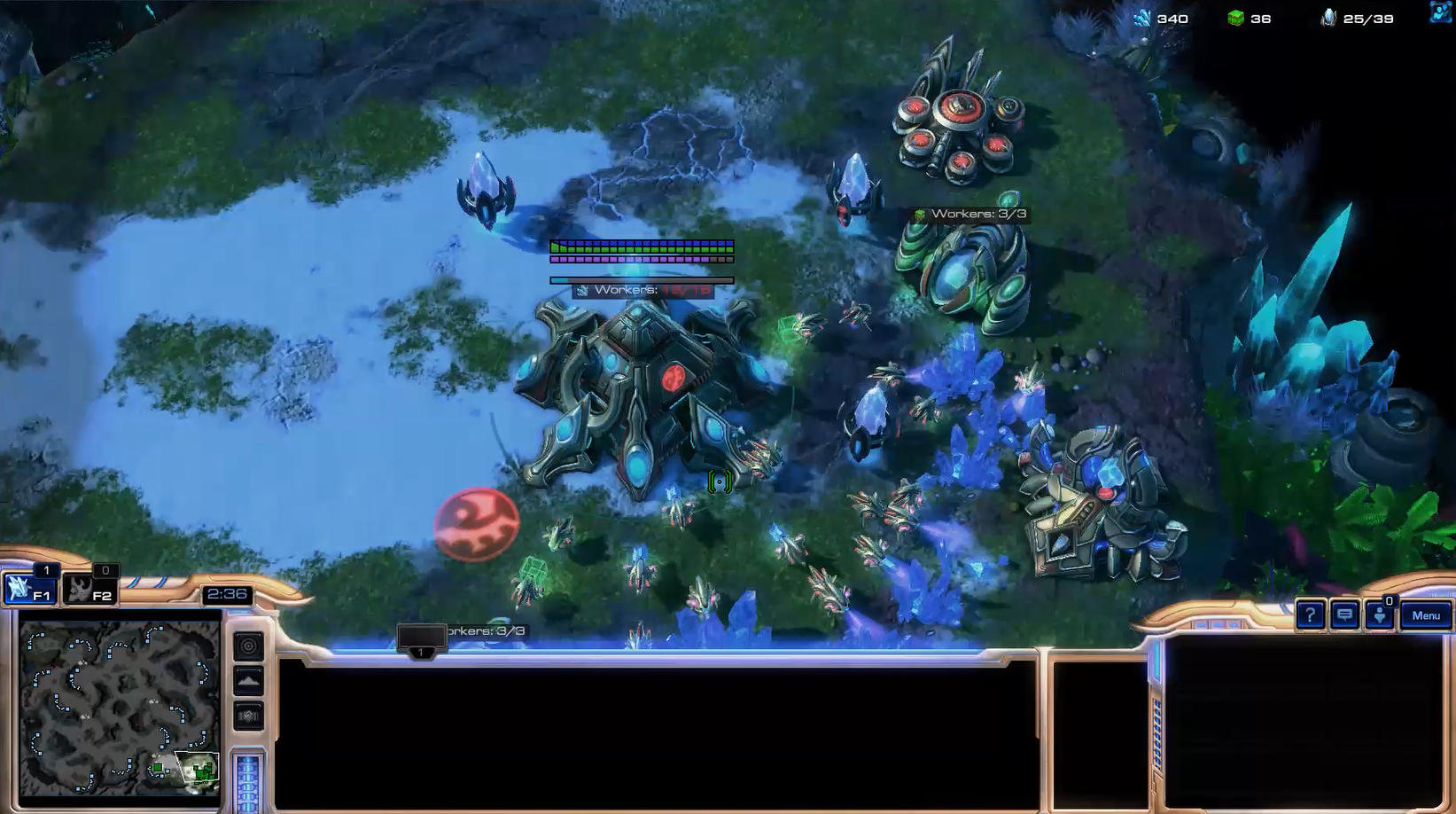
During an internship with Johns Hopkins University, she trained AI agents in the video game StarCraft II in goal-oriented action programming. This AI technique involves dynamic planning with a sequence of actions that activates different goals depending on the progression of the AI within the game.
To continue expanding her opportunities in AI, Sophia worked on a computer vision project using drones to recognize lost or injured persons in collaboration with rescue personnel. The model recognizes someone drowning in a river or finds someone through obscuring objects or terrain. Sophia has used similar computer vision techniques to partner with researchers in Australia to identify invasive grass species.
After a long and winding journey, Sophia feels as though she is finally starting to find a niche at the intersection of ecology and machine learning. Her hope is to work on developing technologies to not only combat issues like the biodiversity crisis, but also to equip farmers with easier methods to manage crops and diagnose diseases. Through her work in this field, she hopes to mitigate issues that farmers currently face and help them through her work in artificial intelligence and machine learning.
Although Sophia’s background was unconventional for a computer science Ph.D. student, she believes that it was her drive to teach herself the material and her deep curiosity to learn and understand the phenomena that she was unfamiliar with that allowed her to progress in the field of AI. She also praises her peers, who took the time to explain challenging concepts and make her transition into the graduate curriculum as seamless as possible.
The learning curve was undoubtedly a steep one. Still, she believes that the barrier to entry was more difficult in perception than in reality and that it was feasible with the right resources and training. So despite having no coding background, she was able to overcome her lack of a traditional background and realize success in her pursuit of a career in AI.
Sophia took the road less traveled and made decisions that many questioned. Still, she followed her heart and discovered newfound passions for ecology, machine learning, and AI. Her previous experiences guided her to what she really wanted to pursue, and it turned out to be one of the most rewarding decisions for her—both personally and professionally.
Join us at GTC 2022 to hear more from Sophia and her colleagues at the panel session, Enabling Unconventional Applications Using AI: A Unique Perspective on September 20.
Curious to know more about working in the field of AI? Check out How to Start a Career in AI for a few key tips. Then get started with free, on-demand NVIDIA AI essentials that will equip you with the fundamentals of AI, data science, graphics, and robotics.
 Embeddings play a key role in deep learning recommender models. They are used to map encoded categorical inputs in data to numerical values that can be…
Embeddings play a key role in deep learning recommender models. They are used to map encoded categorical inputs in data to numerical values that can be processed by the math layers or multilayer perceptrons (MLPs).
Embeddings often constitute most of the parameters in deep learning recommender models and can be quite large, even reaching into the terabyte scale. It can be difficult to fit them in a single GPU’s memory during training.
As such, modern recommenders may require a combination of model parallel and data parallel distributed training approaches to achieve reasonable training times, and the best utilization of available GPU compute.
NVIDIA Merlin Distributed-Embeddings, a library for training large embedding based (for example, recommenders) models in TensorFlow 2 enables you to accomplish this easily with just a few lines of code.
With data-parallel distributed training on GPUs, the whole model is replicated on each GPU worker. A batch of data is split among the multiple GPUs during training, and each device independently operates on its own shard of data.
This allows scaling computations to higher quantities of data with larger batches. The gradients calculated during backpropagation are accumulated across all devices using a reduction operation (for example, horovod.tensorflow.allreduce) for a synchronous parameter update.
With model parallel distributed training, the model parameters are split between various workers. This is a more suitable way to distribute large embedding tables. Training requires using an all-to-all communication primitive (for example, horovod.tensorflow.alltoall) such that workers can get access to the parameters that are not in their partition.
In a related previous post, Training a Recommender System on DGX A100 with 100B+ Parameters in TensorFlow 2, Tomasz discussed how distributing embeddings for a 113 billion-parameter DLRM model across multiple NVIDIA GPUs helped achieve a 672x speedup over a CPU-only solution. This significant improvement can potentially bring down training times from days to minutes! This is accomplished by distributing embedding tables through model parallelism and performing the much-smaller math-intensive MLP layer computation through data parallelism.
Compared to storing the embeddings in CPU memory, this hybrid approach enables you to use the high-memory bandwidth of the GPU memory for memory-bound embedding lookups. It also accelerates the MLP layers using the compute powers among several GPU devices. For reference, an NVIDIA A100-80GB GPU has 80 GB HBM2 memory with a bandwidth at over 2 TB/s).
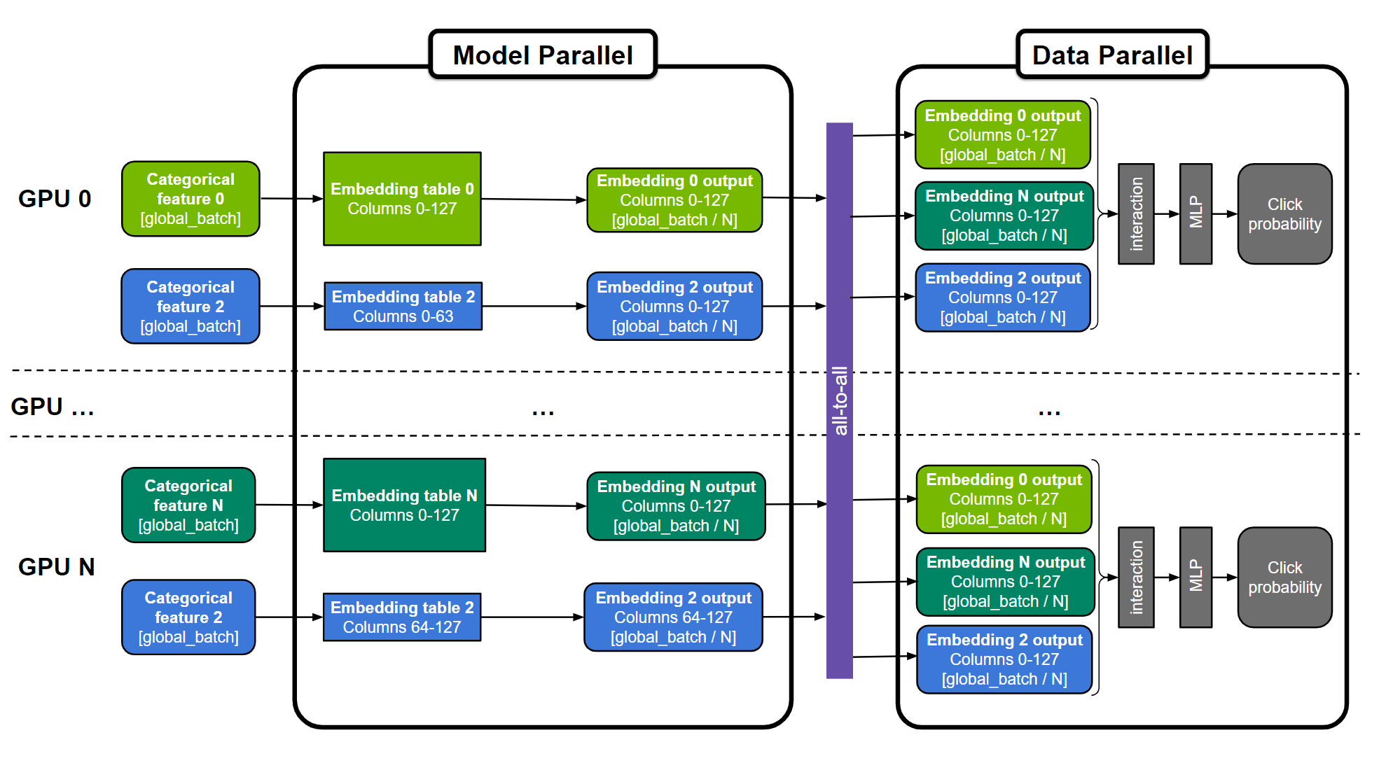
The embedding tables can be split “table-wise” (for example, embedding tables 0 and N), “column-wise” (for example, embedding table 2), or “row-wise”. The MLP layers are replicated across all GPUs. Numerical features can be fed directly into the MLP layers and are not represented in the figure.
However, implementing such a complex hybrid parallel training approach is not trivial and requires a domain expert to engineer several hundred lines of low-level code to develop and optimize training.
To make it more widely accessible, the NVIDIA Merlin Distributed-Embedding library provides an easy-to-use wrapper to democratize model parallelism in TensorFlow 2 with only three lines of Python code. It provides a scalable model parallel wrapper that automatically distributes embedding tables to multiple GPUs, in addition to some efficient embedding operations that cover and extend TensorFlow’s embedding functionalities. Here’s how it enables hybrid-parallelism.
NVIDIA Merlin Distributed-Embeddings provides the distributed_embeddings.dist_model_parallel module. It helps distribute embeddings across several GPU workers without any complex code to handle cross-worker communication with primitives like all2all. The following code example shows the usage of this API:
import dist_model_parallel as dmp

class MyEmbeddingModel(tf.keras.Model):
  def  __init__(self, table_sizes):
    ...
    self.embedding_layers = [tf.keras.layers.Embedding(input_dim, output_dim) for input_dim, output_dim in table_sizes]
    # 1. Add this line to wrap list of embedding layers used in the model
    self.embedding_layers = dmp.DistributedEmbedding(self.embedding_layers)
  def call(self, inputs):
    # embedding_outputs = [e(i) for e, i in zip(self.embedding_layers, inputs)]
    embedding_outputs = self.embedding_layers(inputs)
    ...
To run the dense layers in a data-parallel fashion with Horovod, replace Horovod’s Distributed GradientTape and broadcast methods with their equivalent in Distributed Embeddings. The following example has been taken directly from the Horovod documentation and modified accordingly.
@tf.function
def training_step(inputs, labels, first_batch):
  with tf.GradientTape() as tape:
    probs = model(inputs)
    loss_value = loss(labels, probs)

  # 2. Change Horovod Gradient Tape to dmp tape
  # tape = hvd.DistributedGradientTape(tape)
  tape = dmp.DistributedGradientTape(tape)
  grads = tape.gradient(loss_value, model.trainable_variables)
  opt.apply_gradients(zip(grads, model.trainable_variables))

  if first_batch:
    # 3. Change Horovod broadcast_variables to dmp's
    # hvd.broadcast_variables(model.variables, root_rank=0)
    dmp.broadcast_variables(model.variables, root_rank=0)
  return loss_value
With these minor changes, you are all set with a hybrid-parallel training step!
We also provide complete examples for training a DLRM model with Criteo 1TB click-logs data, as well as synthetic data that scales the model size up to 22.8 TiB.
To demonstrate the benefits of using NVIDIA Merlin Distributed-Embeddings, we show benchmarks on a DLRM model trained on the Criteo 1TB dataset, as well as various synthetic models with up to ~3 TiB embedding table sizes.
Benchmarks indicate that we retain performance similar to expert engineered code with a much simpler API. The NVIDIA DeepLearningExamples DLRM code that uses TensorFlow 2 has now also been updated to leverage hybrid-parallel training with NVIDIA Merlin Distributed-Embeddings. For more information, see our previous post, Training a Recommender System on DGX A100 with 100B+ Parameters in TensorFlow 2.
The benchmarks section in the README provides more insight into performance numbers.
A DLRM model with 113 billion parameters (421 GiB model size) was trained on the Criteo Terabyte Click Logs dataset, over three different hardware setups:
| Hardware | Description | Training Throughput (samples/second) | Speedup over CPU |
| 2 x AMD EPYC 7742 | Both MLP layers and embeddings on CPU | 17.7k | 1x |
| 1 x A100-80GB; 2 x AMD EPYC 7742 | Large embeddings on CPU, everything else on GPU | 768k | 43x |
| DGX A100 (8xA100-80GB) | Hybrid parallel with NVIDIA Merlin Distributed-Embeddings, whole model on GPU | 12.1M | 683x |
We observe that a Distributed-Embeddings solution on a DGX-A100 provides a whopping 683x speedup over a CPU-only solution! We also notice a significant improvement in performance over a single-GPU solution. This is because retaining all the embeddings in GPU memory eliminates the overhead of embedding lookups over the CPU-GPU interface.
To demonstrate the scalability of the solution further, we created synthetic DLRM models of varying sizes (Table 2). For more information about model generation methodology and the training script, see the NVIDIA-Merlin/distributed-embeddings GitHub repo.
| Model | Total number of embedding tables | Total embedding size (GiB) |
| Tiny | 55 | 4.2 |
| Small | 107 | 26.3 |
| Medium | 311 | 206.2 |
| Large | 612 | 773.8 |
| Jumbo | 1,022 | 3,109.5 |
Each synthetic model was trained using one or more DGX-A100-80GB nodes, with a global batch size of 65,536, and the Adagrad optimizer. You can see from Table 3 that NVIDIA Merlin Distributed-Embeddings can easily train terabyte-scale models on hundreds of GPUs.
| Model | Training step time (ms) | ||||
| 1 GPU | 8 GPU | 16 GPU | 32 GPU | 128 GPU | |
| Tiny | 17.6 | 3.6 | 3.2 | ||
| Small | 57.8 | 14.0 | 11.6 | 7.4 | |
| Medium | 64.4 | 44.9 | 31.1 | 17.2 | |
| Large | 65.0 | 33.4 | |||
| Jumbo | 102.3 | ||||
Table 3. Training step time (ms) for synthetic models on various hardware configurations
On the other hand, even for models that can fit into a single GPU, Distributed-Embeddings’ model parallelism still provides substantial speedup with multi-GPU, compared to conventional data parallelism. This is shown in Table 4 where a tiny model runs on DGX A100-80GB.
| Solution | Training step time (ms) | |||
| 1 GPU | 2 GPU | 4 GPU | 8 GPU | |
| NVIDIA Merlin Distributed Embeddings Model Parallel | 17.7 | 11.6 | 6.4 | 4.2 |
| Native TensorFlow Data Parallel | 19.9 | 20.2 | 21.2 | 22.3 |
Table 4. Comparing training step time (ms) for the “Tiny” model (4.2GiB) between an NVIDIA Merlin Distributed Embeddings Model Parallel and a Native TensorFlow Data Parallel solution for embeddings
A global batch size of 65,536 and the Adagrad optimizer were used for this experiment.
In this post, we introduced the NVIDIA Merlin Distributed-Embeddings library, which enables scalable and efficient model-parallel training of embedding-based, deep learning models on NVIDIA GPUs with just a few lines of code. To get started, try the examples for scalable training with synthetic data and training a DLRM model on Criteo data.
 Autonomous vehicle developers now have access to flexible, scalable, and high-performance hardware and software to build the next generation of safer, more…
Autonomous vehicle developers now have access to flexible, scalable, and high-performance hardware and software to build the next generation of safer, more efficient transportation.
NVIDIA DRIVE AGX Orin Developer Kit is now available for general access. Powered by a single Orin system-on-a-chip (SoC), the AI compute platform includes the hardware, software, and sample applications needed to develop production-level autonomous vehicles. It’s also modular, sharing the same design as NVIDIA Jetson, NVIDIA Isaac, and NVIDIA Clara AGX platforms.
With a rich automotive I/O, you have the flexibility to expand and iterate upon your autonomous driving solutions. DRIVE AGX Orin includes a base kit for bench development and an add-on vehicle kit for vehicle installation. The platform also has a smaller footprint than previous generations, with system and accessories included in a single box.
Additionally, NVIDIA DRIVE OS 6 is now available on the NVIDIA DRIVE Developer Download page, providing the latest operating system purpose-built for autonomous vehicles.
NVIDIA DRIVE OS includes NvMedia for sensor input processing, NVIDIA CUDA libraries for efficient parallel computing implementations, and NVIDIA TensorRT for real-time AI inference.
The current version available is DRIVE OS 6.0.4, which supports sensors included in the NVIDIA DRIVE Hyperion 8.1 platform architecture.
You can experience faster downloads and streamlined development environment setup by installing software with NGC DRIVE OS Docker containers or NVIDIA SDK Manager.
DRIVE OS 6.0 provides the following benefits:
For more information, see the NVIDIA DRIVE OS product page.
Before downloading, register for an NVIDIA Developer account and membership in the NVIDIA DRIVE AGX SDK Developer Program. Please submit questions or feedback to the DRIVE AGX Orin general forum.
 Successfully deploying an automatic speech recognition (ASR) application can be a frustrating experience. For example, it is difficult for an ASR system to…
Successfully deploying an automatic speech recognition (ASR) application can be a frustrating experience. For example, it is difficult for an ASR system to correctly identify words while maintaining low latency, considering the many different dialects and pronunciations that exist.
Sign up for the latest Speech AI News from NVIDIA.
Whether you are using a commercial or open-source solution, there are many challenges to consider when building an ASR application.
In this post, I highlight major pain points that developers face when adding ASR capabilities to applications. I share how to approach and overcome these challenges, using NVIDIA Riva speech AI SDK as an example.
Here are a few challenges present in the creation of any ASR system:
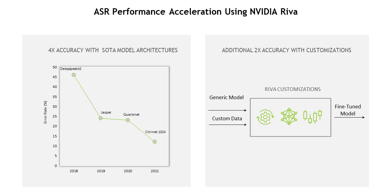
One key metric to measure speech recognition accuracy is the word error rate (WER). WER is defined as the ratio of total incorrect and missing words identified during transcription and sum of total number of words present in the labeled transcripts.
Several reasons cause transcription errors in ASR models leading to misinterpretations of information:
Due to these factors, it is difficult to build a robust ASR model with a low WER score.
A conversational AI application is an end-end pipeline composed of speech AI and natural language processing (NLP).
For any conversational AI application, response time plays a critical factor to make any natural conversations. It would not be practical to converse with a bot if a customer only receives a response after 1 minute of waiting time.
It has been observed that any conversation AI application should deliver a latency of less than 300 msec. So, it becomes critical to make sure that speech AI model latency is far below the 300 msec limit to be integrated into an end-end pipeline for real-time conversational AI applications.
Many factors affect the overall latency of the ASR model:
Optimizing the ASR model and its resource utilizations applies to all AI models and is not only specific to the ASR model. However, it is a critical factor that impacts overall latency as well as the compute cost to run any AI application.
The whole point of optimizing a model is to reduce the inference cost both at compute level as well as the latency level. But all models available online for a particular architecture are not created equally and do not have the same code quality. They also have dramatic differences in performance.
Also, not all of them respond in the same way to knowledge distillation, pruning, quantization, and other optimization techniques to result in improved inference performance without impacting the accuracy results.
Creating an accurate and efficient model is only a small fraction of any real-time AI application. The required surrounding infrastructure is vast and complex. For example, deployment infrastructure should include:
Creating a custom end-end optimized deployment pipeline that supports the required latency requirement for any ASR application is challenging because it requires optimization and acceleration at each pipeline stage.
Based on the number of audio streams that must be supported at a given instance, your speech recognition application should be able to auto-scale the application deployment to provide acceptable performance.
Getting a model to work out-of-the-box is always the goal. However, the performance of currently available models depends on the dataset used during its training phase. Models typically work great for the use case they’ve already been exposed to, but the same model’s performance may degrade as soon as it is deployed in different domain applications.
Specifically, in the case of ASR, the model’s performance depends on accent or language and variations in speech. You should be able to customize models based on the application use case.
For instance, speech recognition models being deployed in healthcare– or financial-related applications require support for domain-specific vocabulary. This vocabulary differs from what is normally used during ASR model training.
To support regional languages for ASR, you need a complete set of training pipelines to easily customize the model and efficiently handle different dialects.
Real-time monitoring and tracking help in getting instant insights, alerts, and notifications so that you can take timely corrective actions. This helps in tracking the resource consumption as per the incoming traffic so that the corresponding application can be auto-scaled. Quota limits can also be set to minimize the infrastructure cost without impacting the overall throughput.
Capturing all these stats requires integrating multiple libraries to capture performance at various stages of the ASR pipeline.
Advanced SDKs can be used to conveniently add a voice interface to your applications. In this post, I demonstrate how a GPU-accelerated SDK like Riva can be applied to solve these challenges when building speech recognition applications.
You can use pretrained Riva speech models in NGC that can be fine-tuned with TAO Toolkit on a custom data set, further accelerating domain-specific model development by 10x.
All NGC models are optimized and sped up for GPU deployment to achieve better recognition accuracy. These models are also fully supported by NVIDIA TensorRT optimization. Riva’s high-performance inference is powered by TensorRT optimizations and served using the NVIDIA Triton Inference Server to optimize the overall compute requirement and, in turn, improve the server throughput
For example, here are a few ASR models on NGC that are further optimized as part of the Riva pipeline for better performance:
Continued optimizations across the entire stack of Riva—from models and software to hardware—has delivered 12x the gain compared to the previous generation.
Latencies and throughput measurements for streaming and offline configurations are reported under the ASR performance section of Riva documentation.
In “streaming low latency” Riva ASR model deployment mode, the average latency (ms) is far less than 50 ms for most of the cases. Using such ASR models, it becomes easier to create a real-time conversational AI pipeline and still achieve the
Deploying your speech recognition application on any platform with ease requires full support. The Riva SDK provides flexibility at each step from fine-tuning models on domain-specific datasets to customizing pipelines. It can also be deployed in the cloud, on-premises, edge, and embedded devices.
To support scaling, Riva is fully containerized and can scale to hundreds and thousands of parallel streams. Riva is also included in the NGC Helm repository, which is a chart designed to automate for push-button deployment to a Kubernetes cluster.
For more information about deployment best practices, see the Autoscaling Riva Deployment with Kubernetes for Conversational AI in Production on-demand GTC session.
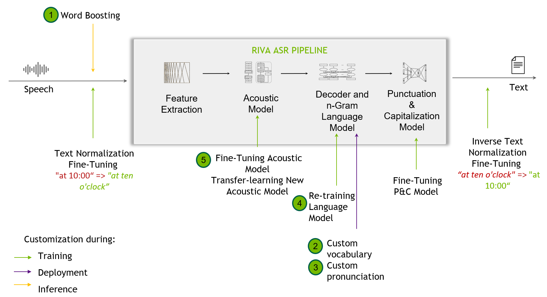
Customization techniques are helpful when out-of-the-box Riva models fall short dealing with challenging scenarios not seen in the training data. This might include recognizing narrow domain terminologies, new accents, or noisy environments.
SDKs like Riva support customization, starting from the word-boosting level, and provision for the end user to custom train their acoustic models.
Riva speech skills also provide high-quality, pretrained models across a variety of languages. For more information about all the models for supported languages, see the Language Support section.
In Riva, underlying Triton Inference Server metrics are available to the end users to use, based on the customization and dashboard creation. These metrics are only available by accessing the endpoint.
NVIDIA Triton provides Prometheus metrics, as well as indicating GPU and request statistics. This helps in monitoring and tracking the production deployment setup.
This post provides you with a high-level overview of common pain points that arise when developing AI applications with ASR capabilities. Being aware of the factors impacting your ASR application’s overall performance helps you streamline and improve the end-to-end development process.
We also shared a few functionalities of Riva that can help mitigate these problems to an extent and even provide customizability tips for ASR applications to support your domain-specific use case.
For more information, see the following resources:
") Register now to experience the most advanced developer tools and learn how experts across industries are using vision AI to increase operational efficiency.
Register now to experience the most advanced developer tools and learn how experts across industries are using vision AI to increase operational efficiency.
Register now to experience the most advanced developer tools and learn how experts across industries are using vision AI to increase operational efficiency.
NVIDIA is collaborating with the United Nations Economic Commission for Africa (UNECA) to equip governments and developer communities in 10 nations with data science training and technology to support more informed policymaking and accelerate how resources are allocated. The initiative will empower the countries’ national statistical offices — agencies that handle population censuses data, economic Read article >
The post UN Economic Commission for Africa Engages NVIDIA to Boost Data Science in 10 Nations appeared first on NVIDIA Blog.