This post is the eighth installment of the series of articles on the RAPIDS ecosystem. The series explores and discusses various aspects of RAPIDS that allow its users solve ETL (Extract, Transform, Load) problems, build ML (Machine Learning) and DL (Deep Learning) models, explore expansive graphs, process signal and system log, or use SQL language … Continued
This post is the eighth installment of the series of articles on the RAPIDS ecosystem. The series explores and discusses various aspects of RAPIDS that allow its users solve ETL (Extract, Transform, Load) problems, build ML (Machine Learning) and DL (Deep Learning) models, explore expansive graphs, process signal and system log, or use SQL language via BlazingSQL to process data.
You may or may not be aware that every bit of information your computer has received from a server miles away, every pixel your screen has shown, or every tune your speakers has produced was some form of a signal that was sent over a ‘wire’. That signal was most likely encoded by the sender end so it could carry the information and the receiver side decoded it for further usage.

Signals are abundant: audio, radio or other electromagnetic waves (like gamma, infrared or visible light), wireless communications, ocean wave, and so on. Some of these waves are man-made, many are produced naturally. Even images or stock market time series can be seen and processed as signals.
cuSignal is a newer addition to the RAPIDS ecosystem of libraries. It is aimed at analyzing and processing signals in any form and is modeled closely after the scikit-learn signal library. However, unlike scikit-learn, cuSignal brings the power of NVIDIA GPUs to signal processing resulting in orders-of-magnitude increase in speed of computations.
Previous posts showcased:
- In the first post, python pandas tutorial we introduced cuDF, the RAPIDS DataFrame framework for processing large amounts of data on an NVIDIA GPU.
- The second post compared similarities between cuDF DataFrame and pandas DataFrame.
- In the third post, querying data using SQL we introduced BlazingSQL, a SQL engine that runs on GPU.
- In the fourth post, data processing with Dask we introduced a Python distributed framework that helps to run distributed workloads on GPUs.
- In the fifth post, the functionality of cuML, we introduced the Machine Learning library of RAPIDS.
- In the sixth post, the use of RAPIDS cuGraph, we introduced a GPU framework for processing and analyzing cyber logs.
- In the seventh post, the functionality of cuStreamz, we introduced how GPUs can be used to process streaming data.
In this post, we will introduce and showcase the most common functionality of RAPIDS cuSignal. As with the other libraries we already discussed, to help with getting familiar with cuSignal, we provide a cheat sheet that can be downloaded here: cuSignal cheatsheet, and an interactive notebook with all the current functionality of cuSignal showcased.
Frequency
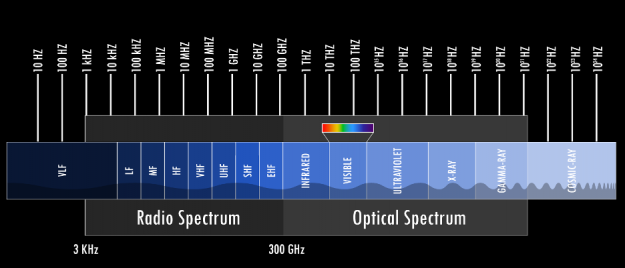
One of the most fundamental properties of signals is frequency. Hertz (abbreviated Hz) is a fundamental unit of frequency defined as a single cycle per second; it was named after Heindrich Rudolf Hertz who provided conclusive proof of the existence of electromagnetic waves. Any signal we detect or store is closely related to time: you could probably safely argue that any signal is a time series with ‘slightly’ different tools to analyze it.
The Alternating Current (AC) supplied to each home is an electric current that oscillates at either 50Hz or 60Hz, audio signals normally cover roughly the spectrum between 20Hz – 20,000Hz (or 20kHz), mobile bands cover some narrow bands in 850-900MHz, 1800Mhz (1.8GHz) and 1900MHz, Wifi signals oscillate at some predefined frequencies around either 2.4GHz or 5GHz. And these are but a few examples of signals that surround us. Ever heard of radio telescopes? The Wilkinson Microwave Anisotropy Probe is capable of scanning the night sky and detecting signals centered around 5 high-frequency bands: 23 GHz, 33 GHz, 41 GHz, 61 GHz, and 94 GHz, helping us to understand the beginnings of our universe. However, this is still just in the middle of the spectrum of electromagnetic waves.
Digital or analog
In the early 20th century, almost all signals we dealt with were analog. Amplifying or recording speech or music was done on tapes and through fully analog signal paths using vacuum tubes, transistors, or, nowadays, operational amplifiers. However, the storage and reproduction of signals (music or else) have changed with the advent of Digital Signal Processing (or DSP). Still, remember CDs? Even if not, the music today is stored as a string of zeros and ones. However, when you play a song, the signal that drives the speaker is analog. In order to play an MP3, the signal needs to be converted from digital to analog and this can be achieved by passing it through the Digital-to-Analog converter (DAC): then the signal can be amplified and played through the speaker. The reverse process happens when you want to save the signal in a digital format: an analog signal is passed through an Analog-to-Digital converter (ADC) that digitizes the signal.
With the emergence of the high-speed Internet and 5th Generation mobile networks, signal analysis and processing has become a vital tool in many domains. cuSignal brings the processing power of NVIDIA GPUs into this domain to help with the current and emerging demands of the field.
Convolution
One of the most fundamental tools to analyze signals and extract meaningful information is convolution. Convolution is a mathematical operation that takes two signals and produces a third one, filtered. In the signal processing domain, convolution can be used to filter some frequencies from the spectrum of the signal to better isolate or detect some interesting properties. Just like in Convolutional Neural Networks, where the network learns different kernels to sharpen, blur or otherwise extract interesting features from an image to, for example, detect objects, the signal convolutions use different windows that help to refine the signal.
Let’s assume that we have a digital signal that looks as below.
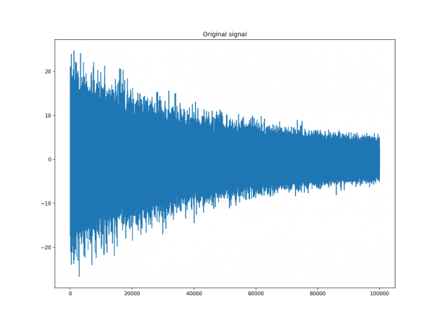
The signal above is a 2 Vrms (Root Mean Squared) a sine wave with its frequency slowly modulated around 3kHz, corrupted by the white noise of exponentially decreasing magnitude sampled at 10 kHz. To see the effect different windows would have on this signal, we will use Hamming and Dolph-Chebyshev windows.
 window_hamming = cusignal.hamming(51)
 window_chebwin = cusignal.chebwin(51, at=100)

 filtered_hamming = cusignal.convolve(
     data
     , window_hamming
     , method='direct'
 ) / cp.sum(window_hamming)

 filtered_chebwin = cusignal.convolve(
     data
     , window_chebwin
     , method='direct'
 ) / cp.sum(window_chebwin)
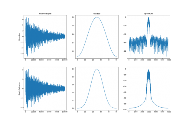
On the right, you can see the difference between the two windows. They are of similar shape but the Dolph-Chebyshev window is narrower and is effectively a more narrow band-pass filter compared to the Hamming window. Both of these methods can definitely help to find the fundamental frequency in the data.
For a full list of all the windows supported in cuSignal, refer to the cheat sheet you can download cuSignal cheatsheet, or try any of them in an interactive cuSignal notebook here.
Spectral analysis
While filtering the signal using convolution might help to find the fundamental frequency of 3KHz, it does not show if (and how) that frequency might change over time. However, spectral analysis should allow us to do just that.
f, t, Sxx = cusignal.spectrogram(x, fs)
plt.pcolormesh(
    cp.asnumpy(t),
    cp.asnumpy(f),
    cp.asnumpy(Sxx)
)
plt.ylabel('Frequency [Hz]')  plt.xlabel('Time [sec]')
The above code produces the following chart:
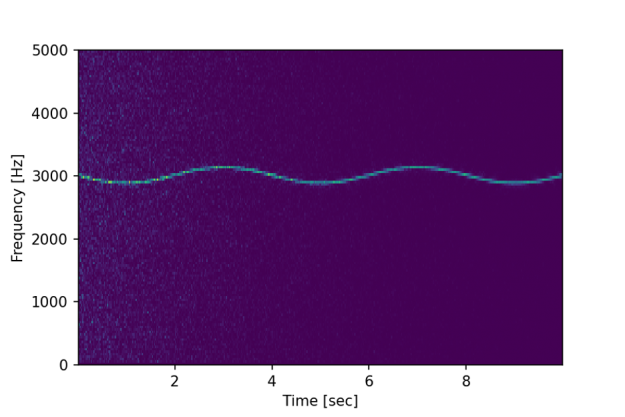
We can now clearly see not only the fundamental frequency of 3kHz is slowly, at 0.25Hz, modulated slightly over time, but we can also observe the initial influence of the white noise shown as lighter blue dots.
With the introduction of cuSignal, the RAPIDS ecosystem gained another great package with a vast array of signal processing tools that can be applied in many domains. You can try the above examples and more for yourself at app.blazingsql.com, and download the cuSignal cheat sheet here!
 Join speakers and panelists considered to be pioneers of AI, technologists, and creators who are re-imagining what is possible in higher education and research.


 Containers have quickly gained strong adoption in the software development and deployment process and has truly enabled us to manage software complexity. It is not surprising that, by a recent Gartner report, more than 70% of global organizations will be running containerized applications in production by 2023. That’s up from less than 20% in 2019. …
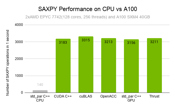
 Back in 2012, NVIDIAN Mark Harris wrote Six Ways to Saxpy, demonstrating how to perform the SAXPY operation on a GPU in multiple ways, using different languages and libraries. Since then, programming paradigms have evolved and so has the NVIDIA HPC SDK. In this post, I demonstrate five ways to implement a simple SAXPY computation …
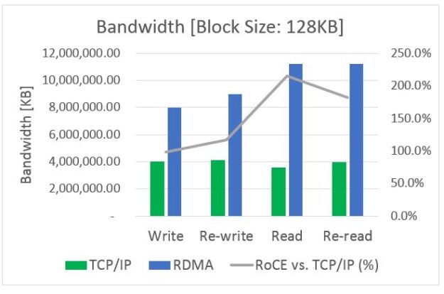
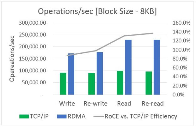
 This post was originally published on the Mellanox blog. Network File System (NFS) is a ubiquitous component of most modern clusters. It was initially designed as a work-group filesystem, making a central file store available to and shared among several client servers. As NFS became more popular, it was used for mission-critical applications, which required access …
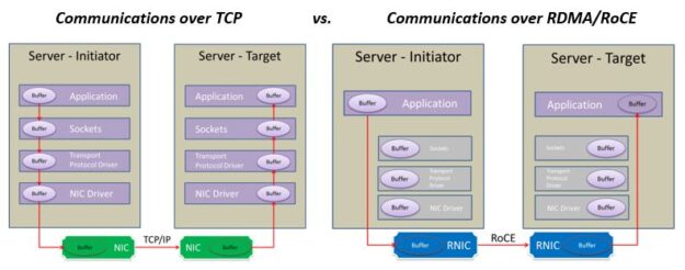
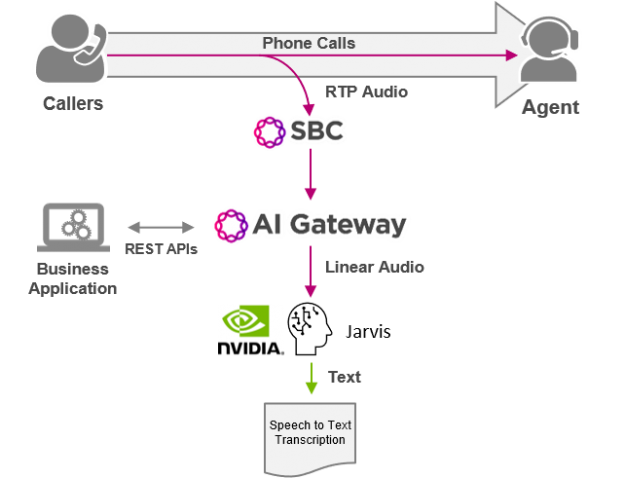
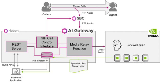
 Many of you may not recognize my company, Ribbon Communications. We are best known for building and securing large telecom networks for communication service providers (also known as phone companies). However, there’s a good chance that in the next day or two, you’ll place a call that traverses a piece of our gear somewhere in …