Reverse time migration (RTM) is a powerful seismic migration technique, providing geophysicists with the ability to create accurate 3D images of the subsurface. Steep dips? Complex salt structure? High velocity contrast? No problem. By splitting the upgoing and downgoing wavefields and combining them with an accurate velocity model, RTM can image even the most complex … Continued
Reverse time migration (RTM) is a powerful seismic migration technique, providing geophysicists with the ability to create accurate 3D images of the subsurface. Steep dips? Complex salt structure? High velocity contrast? No problem. By splitting the upgoing and downgoing wavefields and combining them with an accurate velocity model, RTM can image even the most complex geologic formations.
The algorithm migrates each shot independently using this basic workflow:
Compute the downgoing wavefield.
Reconstruct the upgoing wavefield and reverse it in time.
Correlate up and down wavefields at each image point.
Repeat for all shots and combine in a 3D image.
While simple in concept, the computational costs made RTM economically unviable until the early 2010s, when parallel processing with NVIDIA GPUs dramatically reduced the migration time and hardware footprint needed.
Reducing RTM costs by increasing computational efficiency
There are several factors driving computational requirements for tilted transversely isotropic (TTI) RTM. One is the calculation of first, second, and cross-derivatives along x, y, and z. Earlier versions of GPU, such as the Fermi and Kepler generations, had limited streaming multiprocessors (SMs), shared memory, and compiler technology.
Paulius Micikevicius famously overcame these issues by splitting the derivative calculations into two or three passes, with each pass computing a set of derivatives. This major breakthrough allowed seismic processors to run RTM in an economical and time-efficient manner. However, each pass requires a round-trip to memory. Each round-trip to memory hinders performance and drives up costs.
While multi-pass RTM was the best you could do in 2012, you can do much better today with the NVIDIA Volta or NVIDIA Ampere Architecture generations. If your RTM kernel hasn’t been tuned since the days of Paulius, you are leaving significant value on the table.
Moving to a one-pass RTM
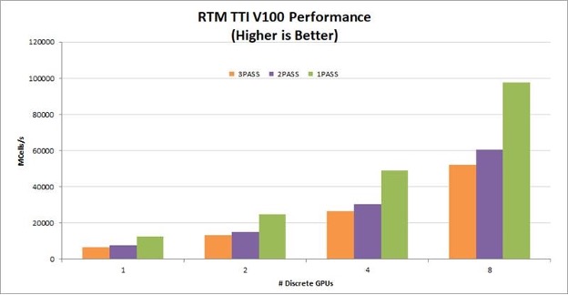
A one-pass TTI RTM kernel reads the wavefield one time, computes all necessary derivatives, and writes the updated wavefields to global memory one time. By eliminating multiple read/write roundtrips to memory, this implementation dramatically increases the performance gained on GPUs. It also helps the algorithm scale linearly across multiple GPUs in a node. Figure 2 shows the performance and strong scaling gained by reducing the number of passes on V100, T4, and A100 GPUs.
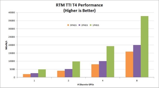
For seismic processing in the cloud, T4 provides a particularly good price/performance solution. On-premises servers for seismic processing typically have four to eight V100 or A100 GPUs per node. For these configurations, reducing the number of passes from three to one improves RTM kernel performance by 78-98%!
Figure 1. A100 performance on multi and single-pass TTI RTM with linear scaling.
Figure 2. T4 performance on multi and single-pass TTI RTM with linear scaling.
Figure 3. V100 performance on multi and single-pass RTM with linear scaling.
Conclusion
Reducing the number of passes in your RTM kernel can dramatically improve code performance and decrease costs. To make the development easier, NVIDIA has developed a collection of code examples showing how to implement a GPU-accelerated RTM using best practices. If we have an NDA in place for you, you can have free access to this code.
Of course, the number of passes in an RTM kernel is only one piece of the puzzle. There are several other tricks shown in the example code to further increase performance, such as compression.
If you’re interested in accessing the NVIDIA RTM implementation or want assistance in optimizing your code, please comment below.
This tutorial is the seventh installment of introductions to the RAPIDS ecosystem. The series explores and discusses various aspects of RAPIDS that allow its users solve ETL (Extract, Transform, Load) problems, build ML (Machine Learning) and DL (Deep Learning) models, explore expansive graphs, process geospatial, signal, and system log data, or use SQL language via … Continued
This tutorial is the seventh installment of introductions to the RAPIDS ecosystem. The series explores and discusses various aspects of RAPIDS that allow its users solve ETL (Extract, Transform, Load) problems, build ML (Machine Learning) and DL (Deep Learning) models, explore expansive graphs, process geospatial, signal, and system log data, or use SQL language via BlazingSQL to process data.
In the age of the Internet, abundant IoT devices, social media, web servers, and more, data flows at incredible speeds. In 2019, Forbes reported that every minute, Americans use approximately 4.4PB of internet data: which converts to roughly 1MB of data per Internet user per minute.
Not only is the volume of data increasing over time, but so are the speeds at which data arrives. Over the years, we went from dial-up modem connections with speeds up to 56kbit in the early 1990s to contemporary 10Gbit networks starting gaining some popularity. 1Gbit networks are still the most widely used type of interconnecting devices at home and in the office unless you are on a WiFi network.
Many of the Internet services offered these days rely on prompt and fast processing of this constant waterfall of data. cuStreamz is one of the newer additions to the RAPIDS stack. It aims to take the streaming data processing historically done on CPU and accelerate on the GPU. Thanks to GPUs’ immense parallelism, processing streaming data has now become much faster with a friendly Python interface.
In the previous posts we showcased other areas:
In the first post, python pandas tutorialwe introduced cuDF, the RAPIDS DataFrame framework for processing large amounts of data on an NVIDIA GPU.
In the sixth post, the use of RAPIDS cuGraph, we introduced a GPU framework for processing and analyzing cyber logs.
Today, we talk about cuStreamz – a library that uses GPUs to process streaming data. To help get familiar with cuStreamz, we also published a cheat sheet that can be downloaded here cuStreamz cheatsheet, and an interactive notebook with all the current functionality of cuStreamz showcasedhere.
Streaming frameworks
First released in 2011, Apache Kafka has quickly become a standard for managing vast quantities of fast-moving data with low latency and high-level APIs. Kafka is a distributed platform that maintains a list of topics that systems can subscribe to (the so-called, consumers), and publish their data onto (the producers). Data in Kafka, like many other distributed systems, is replicated among multiple workers (or brokers): if any of the brokers disconnects from the cluster, or otherwise dies, the data is not lost and still available from other brokers. This improves the resiliency and availability of the system that is required by today’s Internet service companies.
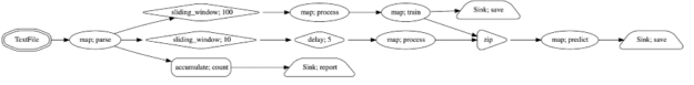
Streamz is a Python framework that focuses on processing high-velocity data and allows for branching, joining, controlling the flow of messages, and sinking the data to disk or other streams. Here’s what a set of distinct pipelines might look like;
The pipeline can branch into multiple branches. A popular Lambda architecture also implements two branches: one to process fast-moving, near real-time data, and another one to provide batch processing.
RAPIDS cuStreamz builds on top of the streamz framework and allows the messages to be batched into cuDF DataFrames instead of text messages. This, on its own, enables significant speed-ups of processing of messages that purport to the same schema by tapping into the power of GPUs. Also, if the data volume cannot fit on a single machine, cuStreams supports pushing the data processing using Dask-cuDF DataFrames.
Setting up locally
It is easy to get started. In this section, we will show you how to set up your own mini-Kafka cluster using Docker. To use cuStreamz, you will, of course, need an NVIDIA GPU with Pascal architecture (GTX 1000-series) or newer as required by RAPIDS.
Next, let’s set up our Kafka cluster. If you clone the Github repository, inside the cheatsheets/cuStreamz folder navigate to Kafka and open docker-compose.yaml file.
Docker-compose uses the YAML configuration files to set up the whole cluster. The first service we start is the zookeeper. Zookeeper is a service used to track naming and configuration data for Kafka; it maintains information about the cluster nodes’ status and their topics, partitions, replication, etc. Besides, the Zookeeper service allows multiple clients to carry out concurrent reads and writes to the service to keep up with the volume and velocity of the incoming and outgoing data calls.
In this example, we use the cp-zookeeper:5.4.3 image from Confluent to start our Zookeeper service; the server started will be named zookeeper. The Zookeeper service can be replicated among multiple servers, so it can become resilient; the Zookeeper servers talk to each other on port 2888, and the leader-of-the-pack runs on port 3888. Clients that want to use the Zookeeper connect to the service on port 2181, and that port gets forwarded to the host via the config ports. We also map some host folders to the container so the data that Zookeeper stores is persisted.
Next, we start two Kafka worker nodes (one shown here for brevity).
The cp-kafka image comes from the Confluent’s Docker Hub; here, we also use version 5.4.3. There are plenty of environmental variables but let’s review just the most important from our point of view:
KAFKA_LISTENERS identifies a list of server names and ports the server will be listening to. Note that the external and internal ports are different: to facilitate communication between multiple docker containers the server will be placed on the Docker internal network (in our case kafka_kafka) and the kafka0 server will be listening on port 19092. If you would like to connect to this service from the host you can use the localhost and port 9092. The same list is provided in the KAFKA_ADVERTISED_LISTENERS environmental variable.
KAFKA_INTER_BROKER_LISTENER_NAME tells the Docker which server name to use for internal communication between containers: in our case, this is LISTENER_DOCKER_INTERNAL but any recognizable name should work. Should you, however, change this name you will have to change the KAFKA_LISTENERS and the KAFKA_ADVERTISED_LISTENERS.
KAFKA_ZOOKEEPER_CONNECT specifies the address of the zookeeper to connect to; in our case, that is zookeeper: 2181.
KAFKA_BROKER_ID is a unique identifier of the kafka node and by convention should be included in the name of the service and server name.
We also identify the zookeeper as a service this container depends on.
To start all these services, simply navigate to the folder where the docker-compose.yaml file is saved and run docker-compose up in the terminal (if you want to stop the service press Ctrl-C or from another terminal window type docker-compose down). Once the services are running, you can check the list of all containers by running docker ps command.
With all the services running, let’s create a sample topic. Run the following command in the terminal.
docker exec -ti bash
Once inside, run the following command.
kafka-topics.sh --create --zookeeper zookeeper:2181 --replication-factor --partitions --topic test
Now, you should be able to subscribe to the topic test to either sink or consume the messages. Your Kafka service is running!!!
Let’s get streaming!
In this example, we will be using the official RAPIDS container. Go ahead and pull the latest one following the examples here https://rapids.ai/start.html. Start the container using the command listed on the RAPIDS website. You should now be able to navigate to https://localhost:8888 and access JupyterLab.
Before we move forward, we need to connect this container to the kafka_kafka network: do so with the following command from the terminal.
docker network connect kafka_kafka
From now on, we should be able to access the kafka0:19092 server from the RAPIDS container.
Note that if you do not have custreamz available in your container, you can install it using the following command.
We will be using the .from_kafka_batched(...) method to subscribe as this allows us to use the CUDA Kafka connector and return the messages in the form of a cudf DataFrame. The first parameter specifies the topic name and is followed by the dictionary with configuration. Next, we set up the interval the stream object will be checking the Kafka topic for new messages; 2 seconds in this example. The engine set cudf specifies that the messages should be returned as DataFrames. We can now provide the rest of the pipeline and start the listener.
from streamz.dataframe import DataFrame

def process_batch(messages):
    batch_df = cudf.DataFrame()

    for message in messages:
        df_split = messages[message].str.tokenize()
        df_split = (
            df_split
            .to_frame('word')
            .reset_index()
            .groupby(by='word')
            .agg({'index': 'count'})
            .rename(columns={'index': 'count'})
            .reset_index()
        )
        print("nWord Count for this batch:")

        batch_df = cudf.concat([batch_df, df_split])

    return batch_df

stream_df = source.map(process_batch)

# Create a streamz dataframe to get stateful word count
sdf = DataFrame(stream_df, example=cudf.DataFrame({'word':[], 'count':[]}))

# Formatting the print statements
def print_format(sdf):
    print("nGlobal Word Count:")
    return sdf

# Print cumulative word count from the start of the stream, after every batch.
# One can also sink the output to a list.
sdf.groupby('word').sum().stream.gather().map(print_format)
After this run;
source.start()
Et voila! We now have a running listener to the test topic!
The code here is pretty self-explanatory, but at the high level, we expect the message to come as a DataFrame. We will count all the words occurring in the message by using the .tokenize() functionality of RAPIDS cudf and then count the number of individual words. Finally, we create a Streamz DataFrame that we use to produce the final tally of words by summing the occurrences of each word.
With the consumer running now, let’s produce some messages! Open a new notebook and install kafka-python package by running in a cell.
The bootstrap_servers is the address of our kafka0 server. Every message we will emit will be JSON string UTF-8 encoded. Now we can start pushing the messages onto the topic message bus:
producer.send('test',{'text': 'RAPIDS rocks!'})
What your notebook with cuStreamz consumer running should produce is a DataFrame with index being RAPIDS and rocks! rows, and a count 1 against each of these words. You can now play more with it!
With the introduction of cuStreamz, the RAPIDS ecosystem can speed up the processing of fast-moving data. You can try the above examples and more for yourself at app.blazingsql.com and download the cuStreamz cheatsheethere.
Jupyter Notebook Best Practices for Using RAPIDS A leading global retailer has invested heavily in becoming one of the most competitive technology companies around. Accurate and timely demand forecasting for millions of item-by-store combinations is critical to serving their millions of weekly customers. Key to their success in forecasting is RAPIDS, an open-source suite of GPU-accelerated libraries. RAPIDS helps them tear through their massive-scale data and … Continued
Jupyter Notebook Best Practices for Using RAPIDS
A leading global retailer has invested heavily in becoming one of the most competitive technology companies around.
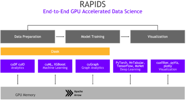
Accurate and timely demand forecasting for millions of item-by-store combinations is critical to serving their millions of weekly customers. Key to their success in forecasting is RAPIDS, an open-source suite of GPU-accelerated libraries. RAPIDS helps them tear through their massive-scale data and has improved forecasting accuracy by several percentage points – it now runs orders of magnitude faster on a reduced infrastructure GPU footprint. This enables them to respond in real-time to shopper trends and have more of the right products on the shelves, fewer out-of-stock situations, and increased sales.
With RAPIDS, data practitioners can accelerate pipelines on NVIDIA GPUs, reducing data operations including data loading, processing, and training from days to minutes. RAPIDS abstracts the complexities of accelerated data science by building on and integrating with popular analytics ecosystems like PyData and Apache Spark, enabling users to see benefits immediately. Compared to similar CPU-based implementations, RAPIDS delivers 50x performance improvements for classical data analytics and machine learning (ML) processes at scale which drastically reduces the total cost of ownership (TCO) for large data science operations.
Figure 1. Data science pipeline with GPUs and RAPIDS.
To learn and solve complex data science and AI challenges, leaders in retail often leverage what are called ‘Kaggle competitions’. Kaggle is a platform that brings together data scientists and other developers to solve challenging and interesting problems posted by companies. In fact, there have been over 20 competitions for solving retail challenges within the past year.
Leveraging RAPIDS and best practices for a forecasting competition, NVIDIA Kaggle Grandmaster Kazuki Onodera won 2nd place in the Instacart Market Basket Analysis Kaggle competition using complex feature engineering, gradient boosted tree models, and special modeling of the competition’s F1 evaluation metric. Along the way, we documented the best practices for ETL, feature engineering, building and customizing the best models for building an AI based Retail forecasting solution.
This blog post will walk readers through the components of a Kaggle competition to explain data science best practices for improving forecasting in retail. Specifically, the blog post explains the Instacart Market Basket Analysis Kaggle competition goals, introduces RAPIDS, then offers a workflow to show how to explore the data visually, develop features, train the model, and run a forecasting prediction. Then, the post will dive into some advanced techniques for feature engineering with model explainability and hyperparameter optimization (HPO).
For an even more detailed look into the methodology, see Kazuki Onodera’s fantastic interview with Medium.com.
Access this Jupyter notebook, where we share these best practices for GPU-accelerated forecasting within the context of the Instacart Market Basket Analysis Kaggle competition.
The Forecasting Challenge
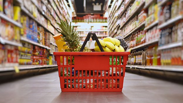
Instacart Market Basket Analysis competition challenged Kagglers to predict which grocery products a consumer will purchase again and when. Imagine, for example, having milk ready to be added to your cart right when you run out, or knowing that it’s time to stock up again on your favorite ice cream.
This focus on understanding temporal behavior patterns makes the problem fairly different from standard item recommendation, where user needs and preferences are often assumed to be relatively constant across short windows of time. Whereas Netflix might be fine assuming you want to watch another movie like the one you just watched, it’s less clear that you’ll want to reorder a fresh batch of almond butter or toilet paper if you bought them yesterday.
Problem Overview
The goal of this competition was to predict grocery reorders: given a user’s purchase history (a set of orders, and the products purchased within each order), which of their previously purchased products will they repurchase in their next order?
The problem is a little different from the general recommendation problem, where we often face a cold start issue of making predictions for new users and new items that we’ve never seen before. For example, a movie site may need to recommend new movies and make recommendations for new users.
The sequential and time-based nature of the problem also makes it interesting: how do we take the time since a user last purchased an item into account? Do users have specific purchase patterns and do they buy different kinds of items at different times of the day?
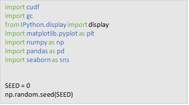
To get started, we’ll first load some of the modules we’ll be using in this notebook and set the random seed for any random number generator we’ll be using.
RAPIDS Overview
Data scientists typically work with two types of data: unstructured and structured. Unstructured data often comes in the form of text, images, or videos. Structured data – as the name suggests – comes in a structured form, often represented by a table or CSV. We’ll focus the majority of the tutorials on working with these types of data.
There are many tools in the Python ecosystem for structured, tabular data but few are as widely used as pandas. pandas represents data in a table and allows a data scientist to manipulate the data to perform a number of useful operations such as filtering, transforming, aggregating, merging, visualizing, and many more.
pandas is fantastic for working with small datasets that fit into your system’s memory. However, datasets are growing larger and data scientists are working with increasingly complex workloads – the need for accelerated compute arises.
cuDF is a package within the RAPIDS ecosystem that allows data scientists to easily migrate their existing pandas workflows from CPU to GPU, where computations can leverage the immense parallelization that GPUs provide.
Getting familiar with the data
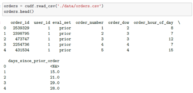
The dataset for this competition contains several files capturing orders from Instacart users over time, with the goal of the competition to predict if a user will re-order a product and specifically, which products will those customers will re-order. From the Kaggle data description (https://www.kaggle.com/c/instacart-market-basket-analysis/data), we see that we have over three million grocery orders with a customer base of over 200,000 Instacart users. And that for each user, we are provided between 4 and 100 of their orders, with the sequence of products purchased in each order as well as the time of their orders and a relative measure of time between orders. Also provided are the week and hour of the day the order was placed, and a relative measure of time between orders.
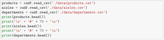
Our products, aisles, and departments datasets are composed of metadata about our products, aisles, and departments respectively. Each dataset (products, aisles, departments, and orders, etc.) has a unique identifier mapping for each entity in that dataset e.g. order_id represents a unique order within the orders dataset, product_id represents a unique product within the products dataset, etc. We’ll use these unique identifiers later to combine all of these separate datasets into one coherent view for exploratory data analysis, feature engineering, and modeling.
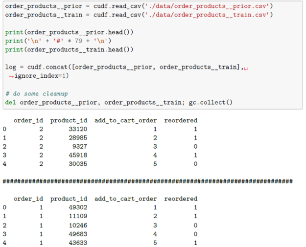
Below, we will read in our data and inspect our different tables using cuDF.
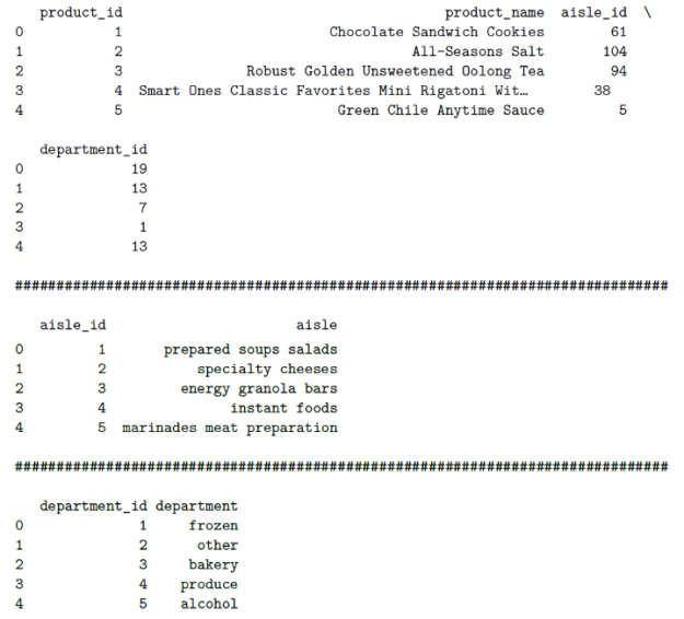
Additionally, we’ll read in our orders datasets. The first indicates to which set (prior, train, test) an order belongs. Additional files specify which products were purchased in each order. Again, from the Kaggle description of the data, we see that the order_products__prior.csv contains previous order contents for all customers. And that the column ‘reordered’ indicates that the customer has a previous order that contains the product. We are informed that some orders will have no reordered items.
Exploring the data
When we think about our data science workflow, one of the most important steps is Exploratory Data Analysis. This is where we examine our data and look for clues and insights into which features we can use (or need to create) to feed our model. There are many ways to explore the data and each Exploratory Data Analysis is different for each problem – however, it still remains incredibly important as it informs our feature engineering process, ultimately determining how accurate our model will be.
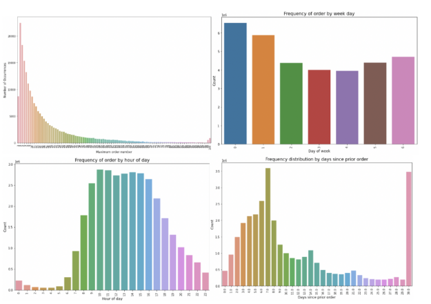
In the notebook, we look at a couple different cross sections of the day. Specifically, we examine the distribution of the order counts, the days of week and times customers typically place orders, the distribution of number of days since the last order, and the most popular items across all orders and unique customers (de-duplicating so as to ignore customers who have a “favorite” item that they place repeated orders for).
Figure 2. Exploring the data
From this we see respectively that:
There are no orders less than 4 and max is capped at 100.
The orders are high Saturday and Sunday (days 0 and 1) and low during Wednesday.
The majority of orders are made during the daytime. And customers primarily order once a week or month (see the peaks at days 7 and 30).
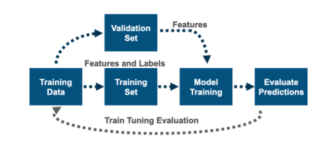
If Exploratory Data Analysis is the most important part of our data science workflow, Feature Engineering is a close second. This is where we identify which features should be fed into the model and create features where we believe they might be able to help the model do a better job of predicting.
Figure 3: Machine Learning is an iterative process.
We start by just identifying our unique User X Item combinations and sorting them. We’ll create a dataset where each user maps to their most recent order number, day of week and hour, and how many days it’s been since that order. And we’ll extend our dataset, creating labels and features to be used later in our machine learning model, such as:
How many kinds of products have the user ordered?
How many products have the user ordered within one cart?
From which departments have the user-ordered products?
When has the user ordered products (day of the week)?
Has this user ordered this product at least once before?
How many orders have a user placed that have included this item?
Solving for the business problem (train and predict)
The mathematical operations underlying many machine learning algorithms are often matrix multiplications. These types of operations are highly parallelizable and can be greatly accelerated using a GPU. RAPIDS makes it easy to build machine learning models in an accelerated fashion while still using a nearly identical interface to Scikit-Learn and XGBoost.
There are many ways to create a model – one can use Linear Regression models, SVMs, tree-based models like Random Forest and XGBoost, or even Neural Networks. In general, tree-based models tend to work better with tabular data for forecasting than Neural Networks. Neural Networks work by mapping the input (feature space) to another complex boundary space and determining what values should belong to those points within that boundary space (regression, classification). Tree-based models on the other hand work by taking the data, identifying a column, and then finding a split point in that column to map a value to, all the while optimizing the accuracy. We can create multiple trees using different columns, and even different columns within each tree.
In addition to their better accuracy performance, tree-based models are very easy to interpret (important for when predictions or decisions resulting from the predictions must be explained and justified, maybe for compliance and legal reasons e.g. finance, insurance, healthcare). Tree-based models are very robust and work well even when there is a small set of data points.
In the section below, we’ll set the different parameters for our XGBoost model and train five different models – each on a different subset of users to avoid overfitting to a particular set of users.
Once we’ve trained our models, we might want to look at the internal workings and understand which of the features we’ve crafted are contributing the most to the predictions. This is called Feature Importance. One of the advantages for tree-based models for forecasting is that understanding the differing importance of our features is very easy.
With understanding how our features contribute to the model accuracy, we can choose to remove features that aren’t important or try to iterate and create new features, re-train, and re-assess if those new features are more important. Ultimately, being able to iterate quickly and try new things in this workflow will lead to the most accurate model and the greatest ROI (for forecasting, oftentimes cost-savings from reduced out-of-stock and poorly placed inventory). Iteration traditionally can take a significant amount of time due to computational intensity. RAPIDS allows users to churn through model iteration with NVIDIA accelerated computing so users can iterate quickly and determine the best performing model.
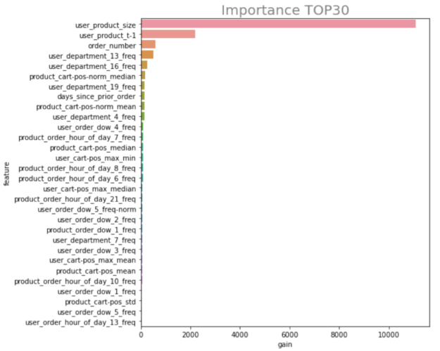
In the Feature Importance section of the notebook, we define convenience code to access the importance of the features in each model. We then pass in our list of models that we trained, iterate over them one by one, and average the importance of each variable across all the models. Lastly, we visualize feature importance using a horizontal bar chart.
We see specifically that three of our features are contributing the most to our predictions:
user_product_size – How many orders has a user placed that has included this item?
user_product_t-1 – Has this user ordered this product at least once before?
order_number – The number of orders that user has created.
Figure 4: Determining top features.
All of this makes sense and aligns with our understanding of the problem. Customers who have placed an order for an item before are more likely to repeat an order for that product, and users who place multiple orders of that product are even more likely to re-order. Additionally, the number of orders a customer has created correlates with their likelihood of re-ordering.
The code uses the default XGBoost implementation of feature importance – but we are free to choose any implementation or technique. A wonderful technique (also developed by anNVIDIA Kaggle Grandmaster, Ahmet Erdem) is called LOFO.
From the description of the LOFO GitHub page, we see that LOFO (Leave One Feature Out) Importance calculates the importance of a set of features based on a metric of choice, for a model of choice, by iteratively removing each feature from the set, and evaluating the performance of the model, with a validation scheme of choice, based on the chosen metric. And that LOFO first evaluates the performance of the model with all the input features included, then iteratively removes one feature at a time, retrains the model, and evaluates its performance on a validation set.
This methodology allows us to effectively determine which features are important for the model. LOFO has several advantages compared to other importance types:
It does not favor granular features.
It generalizes well to unseen test sets.
It is model agnostic.
It gives negative importance to features that hurt performance upon inclusion.
Of these, only a few may be changed and effect the accuracy of our model: max_depth, eta, colsample_bytree, and subsample. However, these may not be the most optimal parameters. The art and science of identifying and training models with the model optimal hyperparamers is called hyperparameter optimization.
While there is no magic button one can press to automatically identify the most optimal hyperparameters, there are techniques that allow you to explore the range of all possible hyperparameter values, quickly test them, and find values that are closest.
A full exploration of these techniques is beyond the scope of this notebook. However, RAPIDS is integrated into many Cloud ML Frameworks for doing HPO as well as with many of the different open source tools. And being able to use the incredible speedups from RAPIDS allows you to go through your ETL, feature engineering, and model training workflow very quickly for each possible experiment – ultimately resulting in fast HPO explorations through large hyperparameter spaces and a significant reduction in Total Cost of Ownership (TCO).
Conclusion
In this blog, we walked through the components of a Kaggle competition to explained data science best practices for improving forecasting in retail. Specifically, the blog post explained the Instacart Market Basket Analysis Kaggle competition goals, introduced RAPIDS, then offered a workflow to show how to explore the data visually, develop features, train the model, and run a forecasting prediction.Then, the post reviewed techniques for feature engineering with model explainability and hyperparameter optimization (HPO).
To learn more, be sure to:
See this Jupyter notebook on forecasting where we show best practices for GPU accelerated forecasting within the context of the Instacart Market Basket Analysis Kaggle competition in which NVIDIA Kaggle Grandmaster Kazuki Onodera won 2nd place, using complex feature engineering, gradient boosted tree models and special modeling of the competition’s F1 evaluation metric.
Recently, one of Sweden’s largest banks trained generative adversarial neural networks (GANs) using NVIDIA GPUs as part of its fraud and money-laundering prevention strategy. Financial fraud and money laundering pose immense challenges to financial institutions and society. Financial institutions invest huge amounts of resources in both identifying and preventing suspicious and illicit activities. There are … Continued
Recently, one of Sweden’s largest banks trained generative adversarial neural networks (GANs) using NVIDIA GPUs as part of its fraud and money-laundering prevention strategy. Financial fraud and money laundering pose immense challenges to financial institutions and society. Financial institutions invest huge amounts of resources in both identifying and preventing suspicious and illicit activities. There are large institutions reportedly saving $150 million in a single year through the use of AI fraud detection.
Existing approaches to identifying financial fraud and money laundering rely on databases of human-engineered rules that match suspicious patterns in financial transactions. As new schemes are identified, new rules are added to the rules base.
Swedbank has developed new solutions to these problems using combinations of deep learning techniques on GPUs, producing new state-of-the-art solutions for identifying suspicious activities. The approach is to model problems in a semi-supervised fashion using anomaly detection via GANs. The solution requires software and hardware that can scale to process and train models on large volumes of data. Hopsworks has trained models on a dataset as large as 40 terabytes (TBs) in size. To this end, the Hopsworks software platform was used with NVIDIA V100 GPUs to engineer features at scale and efficiently train GANs using many GPUs in parallel.
Rules-based vs. model-based fraud detection
Existing approaches to identifying fraud and money laundering rely on databases of human-engineered rules that attempt to match patterns that are indicative of fraud. As new fraud schemes are identified, new rules are added to the rule engines. For example, in money laundering, there are well-known patterns of smurfing money at lots of accounts and aggregating that money using small, under-the-radar transactions at hubs for later spending.
In the Rules-Based Fraud Detection code example, you can see the rule-based approach to identifying suspicious financial transactions. Here, you define a large set of rules that are applied to all financial transactions. If a transaction matches any of the rules, an alert is triggered. If the alert was incorrectly triggered (false positive), it induces costs. If no alert was triggered, but one should have been (false negative), you must design a new rule to identify the fraud scheme. Companies maintain these rule databases and routinely ship updates to customers.
Rules-Based Fraud Detection

# Rule 1
IF transfersLastDay > 10 && amount > $5k
THEN
 alert
END

# Rule 2
IF country is LISTED && amount > $1k
THEN
 alert
END
…
# Rule N
…
Train Fraud Detection Model

dataset=tf.data(“financial_transactions”)
model = …
model.compile(…)
model.fit(dataset, …)

Detect Fraud with Model

IF model.predict(amount,transfersLastDay,
           country, ….) == TRUE
THEN
 alert
END
Given enough historical financial transaction data, model-based approaches are better at pattern matching than rule-based approaches, as they can generalize to learn fraud schemes that are like existing fraud schemes. In the Train Fraud Detection Model code example, you can see that you must first curate a labeled training dataset: financial_transactions. With that dataset, you can train the model and then the trained model can then be used on new financial transactions to predict if they are fraud or not-fraud. An alert is sent if a financial transaction is suspected of fraud.
GANs are a natural choice for financial fraud prediction as they can learn the patterns of lawful transactions from historical data. For every new financial transaction, the model computes an anomaly score; financial transactions with high scores are labeled as suspicious transactions.
GANs are difficult to both train and deploy in production, needing lots of GPUs and parallel hyperparameter search as well as distributed training support. Great care must be exercised and advanced machine learning experience is certainly desired. One of the GAN implementations is based on the Unsupervised Learning of Anomaly Detection from Contaminated Image Data using Simultaneous Encoder Training paper, which describes a architecture for anomaly detection that tolerates small amounts of incorrectly labeled samples and supports parallel encoder training.
Understanding fraud using a graph representation of entities and transactions
To detect fraudulent patterns and trigger alerts, you can use graph and tabular features and the DL-based GAN techniques described earlier. Graphs consist of nodes, also known as vertices, and edges, also known as arcs. In financial applications, graphs can model transactional interactions of businesses and individuals.
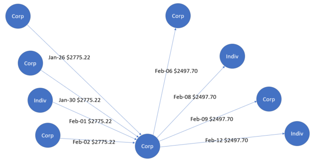
To show the utility of graphs, here’s an example. Mark the businesses and individuals with different titles: businesses are marked as “Corp” and individuals are marked as “Indiv”. The edges are used to represent transactions with associated dates and amounts and the arrows represent the direction of transactions.
There are various expected graph patterns, such as a normal scatter pattern, also known as a dandelion, that happens when an organization pays salaries. Such a pattern occurs on certain dates, salaries are relatively fixed, and the money flow is outbound from a single payer. An anomalous scatter pattern has a sudden burst of transactions that has never been seen previously for involved nodes or bidirectional money flows.
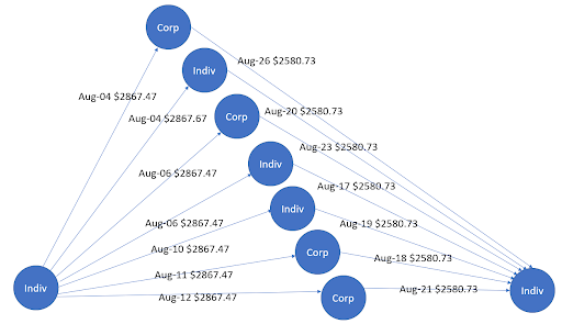
Figure 1 shows a gather-scatter pattern, where money flows initially inbound to the central node in the month of January. These flows are subsequently outbound to other nodes in the month of February. In the world of money-laundering, this gather-scatter pattern is used to hide the distribution of funds from financial institutions. Similarly, Figure 2 shows a scatter-gather pattern that again has a bidirectional flow of money on different dates. In this case, the source and destination of the money are two different central entities.
Figure 1. Gather-scatter pattern through a central entity.
Figure 2. Scatter-gather pattern through two central entities. Outflow occurs before August 17 and inflow thereafter.
Based on tabular features as well as graph features, DL-based GAN methods can detect such fraud patterns, with an example based on using Hopsworks on NVIDIA GPUs. Such methods coexist with rule-based techniques to lead to better results, accuracy, and a confusion matrix.
Challenges in modelling fraud as a binary classification problem
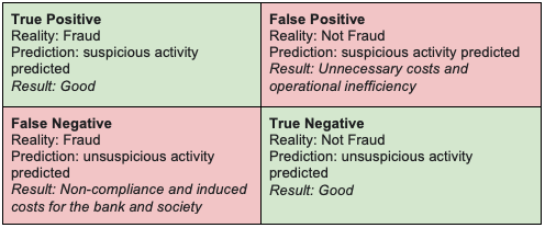
Figure 3 shows the confusion matrix of a financial fraud binary classifier. For problems such as money laundering, false negatives should be weighed significantly higher. Use a variant of the F1 score to evaluate models: precision, recall, and fallout should not be weighted equally.
Figure 3. Confusion matrix of a financial fraud binary classifier.
There are other challenges in detecting money laundering patterns:
Massive class imbalance—Transactions labeled as suspicious may be less than 0.0001% of total historical transactions.
Non-stationarity—New money-laundering schemes are constantly being invented. To identify new patterns as they appear, techniques must be able to adapt themselves or be easily adapted.
Feature engineering programs to compute complex features such as graph embedding and store them in a feature store
Notebooks to find good hyperparameters for the GANs
Distributed training of a GAN using many GPUs.
The code can be reproduced on any Hopsworks cluster, including managed Hopsworks clusters available on AWS, Microsoft Azure, and on-premises installations of Hopsworks with NVIDIA GPUs. Hopsworks clusters can manage up to thousands of GPUs and allocate them to applications on-demand.
NVIDIA GPUs for accelerating financial data science
Identifying fraud and money laundering among large numbers of customer records is a classic financial machine learning (ML) and deep learning (DL) use case. Because it requires many trillion floating point operations (TOPS), applying GPUs accelerates the neural network training process significantly. Many data scientists know that NVIDIA GPUs have been helping in the ML training process for several years.
When the neural network training is complete and the inference phase becomes more important, the recently introduced open-source software NVIDIA Triton Inference Server can help simplify and manage inference acceleration and production model deployment. Triton Server can run as a Docker container, on bare metal, or inside a virtual machine in a virtualized environment. Hopsworks supports serving models on Triton Server using KFServing.
Hopsworks supports ML/DL training using TensorFlow, PyTorch, and Scikit-Learn with additional support for transparent data-parallel training, hyperparameter tuning, and parallel ablation studies on TensorFlow and PyTorch using the Maggy framework. Hopsworks works with multi-GPU, single-node systems as well as clusters of multi-GPU systems. DGX A100 systems are now the universal systems for AI infrastructure for distributed training on the GPU. Each DGX A100 system provides the following configuration:
Multi-GPU, multi-node DGX A100 systems constitute superpods on the Hopsworks platform, which can accelerate DL training and inferencing workloads considerably. You can achieve similar configurations on NVIDIA GPUs by working with the NVIDIA Partner Network (NPN) of OEM partners, system integrators, and value-added resellers.
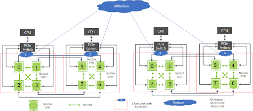
Figure 4 shows the architecture of DL systems using Hopsworks that can leverage data-parallel distributed GPU training using TensorFlow CollectiveAllReduceStrategy. The Maggy framework, supported in Hopsworks, facilitates the ease of development with TensorFlow CollectiveAllReduceStrategy on multi-GPU, multi-node systems, through the transparent management of distribution using Spark. Large clusters additionally benefit from GPU interlinks using NVSwitch. In the future, such an architecture will also be possible using the NVIDIA Rapids.ai framework and Spark on GPUs.
Optimizing distributed training using Hopsworks on NVIDIA-certified multi-GPU, multi-node systems
Figure 4. Multi-GPU, multi-node architecture to train GANs for the anomaly detection task. Note the places where NVLINK is used for high bandwidth.
For inferencing of trained models using other architectures, NVIDIA supports multiple inferencing workloads, concurrent applications, and instances of DL models with the NVIDIA Triton Inferencing Server framework, increasing GPU utilization. Hopsworks clients have used GANs, vision, and other DL models requiring extensive distributed training on the GPU to develop cutting-edge AI systems.
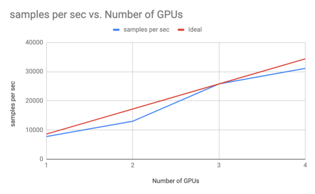
In the following end-to-end money-laundering example from LogicalClocks, a GAN model for anomaly detection was trained on DGX systems using a setup on a multi-GPU, multi-node framework. Training times using such setups can provide almost linear scaling, also known as strong scaling, to accelerate your DL training. Also, inferencing of such models using the Triton Server framework can use the GPUs efficiently.
Figure 5. Close to linear speedup when applying NVIDIA V100 GPUs to the problem of GAN training.
You can also use other frameworks including RAPIDS.ai, Spark on GPU, and the NVIDIA GRAPH framework CuGraph for accelerating such features on the GPU on the Hopsworks platform.
Get in touch with us
Teamwork is the key to engineering accurate financial fraud and money laundering solutions. Going from rule-based to model-based approaches is a common technology objective. The goal is to reduce the number of falsely classified outcomes that financial institutions may receive when using fraud detection or money laundering models in production. Nowadays, customers expect more accuracy from their financial firms in terms of preventing fraud and limiting false alarms.
For more information and to share your experiences with this important use case and state-of-the-art approach, please leave a comment below.
I chose the TensorFlow estimator for implementation due to having a distributed training API support. Well, honestly saying, I found a code, which was quite understandable. So I chose that to implement sensor-based signal recognition on multiple GPUs.
I could not found any solution on google. There might be are multiple issues behind that; implementing in Tensorflow1 can be one of them. I tried to convert that code into Tensorflow2. Mostly code is transformed; however, tf.contrib related things did not restore. So I decided to edit that code for sensor-based signal (Time series).
However, when I ran the code, the accuracy was 30%, and the lost value was bigger. On the other hand, when I implemented CNN on the same data set on Low-level tensor API, I received 95% accuracy. Now I do not know why it is giving low accuracy on the tf estimator. In my opinion, one of the reasons can be wrong input feeding to the CNN. Here is the code:
def cnn_model_fn(features, labels, mode):
“””Model function for CNN.”””
# Input Layer
# Reshape X to 4-D tensor: [batch_size, width, height, channels]
# input 1 * segment_size, and have three channel, in accelrometer we have x, y, z
in `def cnn_model_fn(features, labels, mode):` I am getting {‘x’: <tf.Tensor ‘IteratorGetNext:0’ shape=(?, 600) dtype=float64>} and in labels Tensor(“IteratorGetNext:1”, shape=(?,), dtype=int64) and in mode {str} train.
**Here the result on test data:**
Saving ‘checkpoint_path’ summary for global step 1000: /tmp/tmp77ffy2i9/model.ckpt-1000
I’m looking to put on a project for school, a RNN to predict stock prices (not really innovative i know).
All the programs i see to learn how to make this model has a very strange feedback 50% goes like “you rock this is great” the other 50% goes like “this makes no sense”.
Is this project something hard to do with Keras+TensorFlow?
Any 1 can help me navigate the immensive amount of documents about TF to get me started?
Looking to improve your cloud gaming experience? First, become a master of your network. Twitch-class champions in cloud gaming shred Wi-Fi and broadband waves. They cultivate good ping to defeat two enemies — latency and jitter. What Is Latency? Latency or lag is a delay in getting data from the device in your hands to Read article >
픽사 애니메이션 스튜디오는 아래 이미지에서 낯익은 케릭터들이 많이 있는 만큼, 흥행한 작품들이 굉장히 많은 회사 입니다. 특히 초창기에는 작품을 낼때마다 박스오피스 1위를 할 정도였죠. 어떻게 애니메이션을 만드는지 아는 것이 별로 없지만, 창의성이 중요하다는 것은 알 수가 있습니다. 이런 창의성이 요구되는 활동을 성공적으로, 그리고 꾸준하게 해낼 수 있었던 비결은 무엇일까요?
이 책에는 저자 애드 캣멀이 픽사라는 회사와 함께 성장하는 과정과 애니메이션을 하나하나 성공시켜가면서, 경영자로서 스스로 무수히 많은 질문을 던지고 답을 찾아가는, 이러한 전반적인 과정들이 담겨있습니다. 그 뿐만 아니라 실질적으로 참고할 수 있도록, 픽사에서 실제 진행한 프로세스들에 대한 이야기도 포함되어 있습니다.
저는 이 책을 읽으면서 특히 저자가 경영자로서 계속해서 마주치는 문제들에 대해서 다양한 관점으로 고려하면서 답을 찾아가는 과정이 인상이 깊었습니다. 숫자를 세어본 적은 없지만, 계속해서 물음표로 글이 이어지는 부분들도 적지 않았던 것 같네요.
픽사 사장으로서 내 목표는 언제나 픽사가 창업자들(스티브 잡스, 존 래스터, 그리고 나)보다 오래 생존할 수 있게 픽사에 계속 생명력을 불어놓는 창의적 기업문화를 구축하는 것이었다. 예술과 상업이라는 상호충돌하면서도 상호보완적인 동력을 관리하느라 애를 먹고 있는 경영자들과 창의적 기업문화에 관한 철학을 공유하는 것도 내 목표다. … 나는 어떤 분야에든 사람들이 창의성을 발휘해 탁월한 성과를 내도록 이끄는 훌륭한 리더십이 필요하다고 생각한다.
머리말 – 잃어버리고 되찾은 것 중에서
경영이란 이런 것이다. 타당한 이유에 따라 내린 결정이 새로운 문제를 초래하고, 이 새로운 문제를 해결하기 위해 또 다른 결정을 내려야 한다. 기업에서 발생하는 문제는 최초의 오류를 수정하는 것마으로 간단히 풀리는 법이 없다. 하나의 문제를 해결하는 일은 여러 단계를 거쳐야 하는 과정이다. 최초의 문제뿐만 아니라 여기서 파생된 문제가 무엇인지 파악해 함께 해결해야 한다.
Chapter 1 애니메이션과 기술의 만남
나는 오랫동안 인식의 한계에 대해 고민했다. 경영자는 항상 인식의 한계에 관한 문제로 인해 고민하게 마련이다. 우리는 어디까지 볼 수 있는가? 얼마나 많은 것을 불명확하게 인식하고 있는가? 우리가 카산드라의 경고를 무시하고 있는 건 아닐까? 다시 말해, 우리가 최선을 다해 문제를 파악하려고 노력해도 문제를 인식하지 못하는 저주를 받은 것은 아닐까? 이런 의문들의 답을 찾는 과정은 창의적 기업문화를 유지하는 열쇠다. 그리고 그 답을 탐구하는 것이 이 책의 핵심 내용이다.
Chapter 9 잠재적 위험에 대처하는 법 중에서
이 부분은 애드 캣멀이 어떠한 사람인지를 알 수 있는 대목이기도 합니다.
나는 다른 기업 사람들이 나와 달리 공격적이고 확신에 찬 행동을 하는 것을 보고, 내가 사장답지 않아 보일까 봐 걱정했다. 더 정확히 말하면, 나는 실패가 두려웠다.
나는 연설에서 8~9년 전에야 겨우 내가 사기꾼이 된 것 같은 기분에서 벗어날 수 있었다고 털어놨다. … “자신이 사기꾼처럼 느껴지는 분이 있나요?” 그러면 언제나 모든 직원이 손을 든다.
… 자신이 경영자로서 잘해 나가고 있는지 파악하려면, 머릿속에서 경영자란 어떤 것이어야 한다는 심성모형을 지워야 한다. 경영자의 성공을 측정하는 척도는 ‘팀원들이 잘 협력해 핵심적인 문제들을 해결하고 있는가?’ 이다.
Chapter 6 실패와 공포에 대처하는 법 중에서
제품을 만드는 모두를 위한,
이 책을 추천하는 이유는 픽사라는 회사를 가지고 이야기를 하고 있지만, 제품을 만드는 수 많은 회사들에도 적용할 수 있는 좋은 길잡이이기 때문입니다.
먼저 우리는 그 어느때보다 ‘창의력’이 중요시 되는 시대에 살고 있습니다. ‘지식근로자’라는 말은 1968년 피터드러커가 ≪단절의 시대≫ 을 저술하면서 처음 언급 했었습니다. 이제는 이 지식근로자라는 말이 전혀 낯설지 않은 시대에 우리는 살고 있습니다. 또한 실제로 AI가 급격히 발전하면서 단순 반복적인 일들이 대체되고 있는 상황입니다. 이에 자연스럽게, AI가 잘하지 못하는 일들이 이 지식근로자들에게 요구되고 있습니다. 이러한 일들 중 가장 기본이 되는 것이 무엇일까요? 핵심 요소 중에서 하나가 바로 창의성일 것입니다.
새로운 제품을 만드는데 있어서 이 창의성은 굉장히 중요한 요소입니다. 문제를 발견하고, 어떤 식으로 풀지 이 전반적인 과정에 모두 이 창의성이 활용되기 때문이죠. 그리고 픽사에서 애니메이션을 제작하는 것을 스타트업에서 제품을 만들어내는 것에 비유할 수 있습니다. 흔히 스타트업에서 새로운 제품을 만드는 과정을 다음과 같이 이야기 할 수 있습니다.
고객을 깊이 이해하고, 주어진 문제를 풀어내서, 고객에게 전달하여 감동을 주는 것.
에니메이션을 만드는 과정 또한 비슷한 프레임을 가지고 있습니다.
전달하고자 하는 스토리를 구상하고, 배경과 하나하나의 케릭터에 숨을 불어넣어서, 관객들에게 전달하여 감동을 주는 것.
전달하는 제품의 형태만 다를 뿐, 고객(관객)들에게 감동을 주는 것은 동일하기 때문입니다. 그럼 이 다음부터는 픽사가 어떤 식으로 성장해왔는지 간략하게 다뤄보겠습니다.
픽사의 정체성, 목표와 기업문화 (사람과 프로세스)
먼저 인상 깊었던 부분들 중 하나는 픽사라는 회사의 색깔을 명확하게 한 것입니다. 다음은 회사의 정체성을 구축하는 데 있어 가장 중요한 두가지 요소입니다. 첫 번째가 회사가 추구하는 목표(미션)가 무엇인지, 두 번째로는 기업 문화에 해당합니다. 픽사는 사람들에게 감동을 주는 애니메이션을 만드는 것을 목표로 하였고, 상황에 타협하지 않았고 본질을 계속 추구한 집단이기도 하였습니다.
당시 픽사는 파산 위기에 처한 신생 영화사에 불과했지만, 직원들은 신념을 공유했다. 우리가 보고 싶은 영화를 만들면 관객들도 보러 올 것이라는 신념이었다. 우리는 이 신념을 지키기 위해, 계속해서 커다란 바위를 산꼭대기로 밀어올리는 시시포스처럼 불가능한 일에 무모하게 도전하는 기분을 맛봐야 했다.
… 픽사 임직원이 자부심을 느낀 대목은 이런 숫자가 아니다. 수익은 기업의 성과를 측정하는 여러 가지 잣대 중 하나로, 가장 의미 있는 잣대라고 할 수 없다. 내가 가장 자부심을 느끼는 부분은 우리가 만든 작품의 예술적 성취도다. … 우리가 추구한 진짜 목적은 그때나 지금이나 위대한 영화를 제작하는 것이다.
머리말 – 잃어버리고 되찾은 것 중에서
‘토이 스토리’를 제작하는 과정에서 픽사에 지대한 영향을 미치게 될 두 가지 창작 원칙이 만들어졌다. …
제1원칙은 “스토리가 왕이다(Story is King)” 이다. …
제2원칙은 “프로세스를 신뢰하라(Trust the Process)”다. 우리는 이 원칙을 좋아했다. 제작 과정의 고민을 덜어주는 원칙이기 때문이다.
Chapter 4 픽사의 정체성 구축 중에서
우리는 디즈니 중역들을 만나 극장용보다 질이 낮은 비디오 대여용 애니메이션을 제작하는 일은 픽사의 기업 성향에 맞지 않는다고 말했다. 픽사의 기업문화는 이를 용납하지 못했다. 우리는 진로를 바꾸어 ‘토이 스토리2’를 극장용 애니메이션으로 만들자고 제안했다. 놀랍게도 디즈니 중역들은 흔쾌히 승낙했다.
Chapter 4 픽사의 정체성 구축 중에서
기업문화에 있어서 가장 중요한 요소는 ‘사람’ 입니다. 많은 책들에서 적합한 사람, 인재밀도 등을 언급하는 것처럼, 저자 역시 사람에 대해서 특히 중요하게 여기는 것을 볼 수가 있습니다.
나는 다음과 같은 교훈을 얻었다. 좋은 아이디어를 평범한 팀에 맡기면 실망스러운 결과가 나온다. 반면 평범한 아이디어를 탁월한 팀에 맡기면, 그들은 아이디어를 수정하든 폐기하든 해서 더 나은 결과를 내놓는다.
이 교훈은 더 설명할 가치가 있다. 적합한 팀에게 일을 맡기는 것이 아이디어를 성공적으로 구현하는 선결 조건이다. 재능 있는 인재들을 원한다고 말하기는 쉽고, 경영자들 또한 재능 있는 인재들을 원하지만, 정말로 핵심 관건은 이런 인재들이 상호작용하는 방식이다. 아무리 영리한 사람들을 모아놓아도 서로 어울리지 않으면 비효율적인 팀이 된다. 경여앚가 직원 개개인의 재능이 아니라 팀이 돌아가는 상황에 초점을 맞추는 편이 낫다는 뜻이다. 좋은 팀은 서로 보완해주는 사람들로 구성된다. … 업무에 적합한 인재들이 상성이 맞는 사람들과 함께 일하도록 하는 것이 좋은 아이디어를 내는 것보다 중요하다.
Chapter 4 픽사의 정체성 구축 중에서
한 사람만이 내가 던진 질문에 오류가 있다고 지적했다. 아이디어는 사람에게서 나온다. 사람이 없으면 아이디어도 없다. 따라서 사람이 아이디어보다 중요하다.
왜 사람이 아이디어보다 중요하다고 생각하지 못할까? 너무나 많은 사람이 아이디어가 사람들과 완전히 분리된 채 독립적으로 형성되고 존재한다고 착각하기 때문이다. 아이디어는 독립적인 존재가 아니다. 아니디어는 종종 수십 명이 관여하는 수만 가지 의사결정을 통해 형성된다. … 영화는 하나의 아이디어만으로 만들어질 수 없다. 영화는 여러 아이디어의 집합체다. 이런 아이디어들을 구상하고 현실로 구현하는 것은 결국 사람이다. 모든 제품이 마찬가지다. …
다시 말해, 사람(직원들의 근무 습관, 재능, 가치)에게 초점을 맞추는 것이 모든 창조적 사업의 핵심 성공 비결이다. 제작 과정에서 나는 이런 사실을 이전보다 명확히 인식하게 됐다. .. 이후 픽사는 사람을 우선하는 경영 모델을 꾸준히 실천하고 있다. 세부적인 수정은 있었지만, 근본 원리는 언제나 같다. 좋은 인재를 육성하고 지원하면 그들이 좋은 아이디어를 내놓는다는 것이다.토이>
Chapter 4 픽사의 정체성 구축 중에서
다음으로는 뛰어난 사람들이 각자의 역량을 펼칠 수 있도록, 서로 효율적으로 협력하는 방법들에 대한 고민을 계속 하는 것을 볼 수 있습니다. 이는 제품의 질이 직원들에게 달려있다는 것을 전적으로 믿기 때문이죠.
당시 일본 제조업에서 일어난 품질관리 혁명을 설명하기 위해 적기공급생산(just-in-time manufacturing), 전사적 품질관리(total quality control) 같은 경영학 용어들이 나왔다. 이런 용어들이 설명하려는 아이디어는 간단하다. 즉, 문제를 파악해 수정할 권한을 고위 간부부터 생산라인 말단직원까지 모든 임직원에게 부여해야 한다는 것이다. 에드워드 데밍은 어떤 직급의 직원이라도 제조 과정에서 문제를 발견하면 조립라인을 멈추도록 장려해야 한다고 생각했다. …
에드워드 데밍과 도요타의 접근법은 제품 생산 과정에 밀접하게 관여하는 사람들에게 제품의 품질을 높일 권한과 책임을 부여했다. 이 과정에서 일본 근로자들은 자신이 단지 컨베이어벨트 위를 지나가는 부품들을 조립하는, 영혼 없는 톱니바퀴 같은 존재가 아니라, 제품 생산 과정의 문제를 지적하고, 변화를 제안하고, 문제 해결에 기여해 회사를 키우는 구성원이라는 ‘자부심’을 느꼈다(나는 특히 마지막 대목이 중요하다고 생각한다).
… 에드워드 데밍의 품질관리 이론은 ‘모든 직원은 먼저 허락받지 않은 채, 문제 해결에 나설 수 있어야 한다’ 라는 민주적 원칙에 기반을 두고 있다. … 경영진이 단기이익 극대화에 집착하자 자부심을 가지고 품질 향상에 힘쓰던 직원들은 영혼을 잃은 채 일하게 됐고, 그 결과 품질 결함이 발생하기 시작했다.
Chapter 3 의 탄생과 목표의 재정립 중에서토이>
이러한 고민들의 결과로서 창작 제 2원칙으로 “프로세스를 신뢰하라” 가 있는 것처럼, 픽사에서는 좋은 작품을 만들기 위한 다양한 프로세스를 정립하기 위한 많은 시도들이 있었습니다. 아래는 픽사라는 회사가 어느정도 큰 큐모를 갖춘 이후에 정립된 프로세스을 나열해둔 것 입니다.
데일리스 회의
현장답사
한도 결정
기술과 예술의 융합
소규모 실험
보는 법 배우기
사후분석 회의
픽사대학
프로세스들을 하나하나 보다보면, 이러한 생각이 들기도 합니다. ‘우리도 이런 것들은 하고 있는 거 같은데?’ 하지만 자세히 들여다보면 픽사가 구축해온 기업문화를 기반으로 위 프로세스들이 일반적인 기업들과는 다르게 돌아가는 것을 이해할 수 있습니다. 최근에 읽었던 넷플릭스의 ≪규칙없음≫ 에서 자유와 책임이 주어지는 것처럼, 픽사에서 역시 개개인에게 자유와 책임이 주어지는 것을 느낄 수 있었습니다.
‘픽사의 브레인트러스트가 다른 기업의 피드백 매커니즘과 다른 게 뭐야?’ … 첫째, 픽사의 브레인트러스트는 스토리텔링을 심도 있게 이해하는 사람들, 대게 작품 제작에 참여해본 경험이 있는 사람들로 구성된다. 픽사 감독들은 다양한 사람들의 비평을 환영하지만(사실 모든 픽사 직원들은 중간결과물을 보고 의견서를 보내야 한다), 특히 동료 감독, 각본가가 보낸 피드백을 더 진지하게 받아들인다. 둘째, 픽사의 브레인트러스트는 지시할 권한이 없다. 이는 중요한 차이다. 감독은 브레인트러스트의 특정 제안을 꼭 받아들여야 할 필요가 없다. 브레인트러스트 회의 후, 브레인트러스트의 피드백을 어떻게 받아들일지 결정하는 것은 감독의 몫이다.
Chapter 5 솔직함의 가치 중에서
위의 프로세스 외에도 인턴 프로그램, 전사 워크샵인 노트 데이 등에 대한 이야기가 담겨 있습니다. 특히 노트데이에서는 단순히 직원들의 참여를 유도하는 것이 아니라 토론회가 제대로 돌아갈 수 있도록 설계하는 과정까지 담겨 있어서 흥미롭게 볼 수 있었습니다.
제작비를 10퍼센트 감축하는 방안을 고민하는 자리에서 귀도 쿼로니는 간단한 제안을 했다.
“모든 직원에게 비용 삭감 아이디어를 내달라고 요청합시다.”
존 래스터는 흥분한 얼굴로 말했다. “흥미로운 제안이군요. 하루 동안 모든 픽사 직원의 업무를 중단하고, 이 문제를 해결할 방안을 얘기해보는 게 어떨까요?”
Chapter 13 노트 데이 토론회 중에서
끝으로
수 많은 스타트업을 꿈꾸는 분들에게, 특히 정체성이 명확한 회사를 만들고 싶은 분들에게 좋은 길잡이가 되어줄 책이라고 생각을 합니다. 마지막으로 존 래스터가 기업문화에 대해서 이야기한 문장과 애드 캣멀의 경영자의 목표로 책 소개를 마무리 하고자 합니다.
존 래스터는 종종 픽사의 조직문화를 살아 있는 유기체에 비유했다. “지구상에 출현한 적 없는 새로운 생명체를 키우는 방법을 우리가 발견한 것 같아요.”
이 책을 써내려오면서 내 목표는 픽사와 디즈니 애니메이션 스튜디오 직원들이 어떻게 얼마나 끈질기게 비전을 실현할 방법을 모색했는지 독자들에게 알리는 것이었다. 미래는 목적지가 아니라 방향이다. 우리가 할 일은 현재의 진로가 옳은지 매일 점검하고, 길을 벗어났다면 방향을 수정하는 것이다. … 불확실성과 변화는 변수가 아니라 인생에서 피할 수 없는 상수다. 불확실성과 변화가 있기에 인생이 재미있는 것이다.
원래 경영자의 목표는 달성하기 쉬울 수 없다. 경영자의 목표는 탁월한 제품을 만드는 것이다.

 Reverse time migration (RTM) is a powerful seismic migration technique, providing geophysicists with the ability to create accurate 3D images of the subsurface. Steep dips? Complex salt structure? High velocity contrast? No problem. By splitting the upgoing and downgoing wavefields and combining them with an accurate velocity model, RTM can image even the most complex … Continued
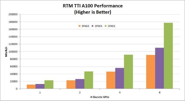
 This tutorial is the seventh installment of introductions to the RAPIDS ecosystem. The series explores and discusses various aspects of RAPIDS that allow its users solve ETL (Extract, Transform, Load) problems, build ML (Machine Learning) and DL (Deep Learning) models, explore expansive graphs, process geospatial, signal, and system log data, or use SQL language via …
 Recently, one of Sweden’s largest banks trained generative adversarial neural networks (GANs) using NVIDIA GPUs as part of its fraud and money-laundering prevention strategy. Financial fraud and money laundering pose immense challenges to financial institutions and society. Financial institutions invest huge amounts of resources in both identifying and preventing suspicious and illicit activities. There are …