Recommender systems (RecSys) have become a key component in many online services, such as e-commerce, social media, news service, or online video streaming. However with the growth in importance, the growth in scale of industry datasets, and more sophisticated models, the bar has been raised for computational resources required for recommendation systems. To meet the … Continued
Recommender systems (RecSys) have become a key component in many online services, such as e-commerce, social media, news service, or online video streaming. However with the growth in importance, the growth in scale of industry datasets, and more sophisticated models, the bar has been raised for computational resources required for recommendation systems.
To meet the computational demands for large-scale DL recommender systems, NVIDIA introduced Merlin – a Framework for Deep Recommender Systems. Now NVIDIA teams have won two consecutive RecSys competitions in a row: the ACM RecSys Challenge 2020, and more recently the WSDM WebTour 21 Challenge organized by Booking.com. The Booking.com challenge focused on predicting the last city destination for a traveler’s trip given their previous booking history within the trip. NVIDIA’s interdisciplinary team included colleagues from NVIDIA’s KGMON (Kaggle Grandmasters), NVIDIA’s RAPIDS (Data Science), and NVIDIA’s Merlin (Recommender Systems) who collaborated on the winning solution.
This post is the second of a three-part series that gives an overview of the NVIDIA team’s first place solution for the booking.com challenge. The first post gives an overview of recommender system concepts. This second post discusses deep learning for recommender systems. The third post will discuss the winning solution, the steps involved, and also what made a difference in the outcome.
Deep Learning for Recommendation
As the growth in the volume of data available to power recommender systems accelerates rapidly, data scientists are increasingly turning from more traditional machine learning methods to highly expressive deep learning models to improve the quality of their recommendations.
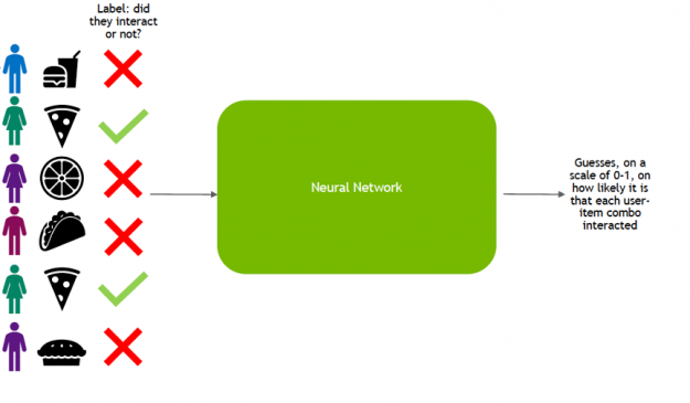
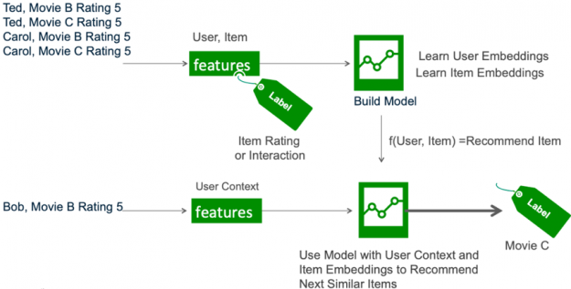
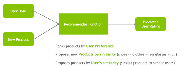
Broadly, the life-cycle of deep learning for recommendation can be split into two phases: training and inference. In the training phase, the model is trained to predict user-item interaction probabilities (calculate a preference score) by presenting it with examples of interactions (or non-interactions) between users and items from the past.
Once it has learned to make predictions with a sufficient level of accuracy, the model is deployed as a service to infer the likelihood of new interactions.
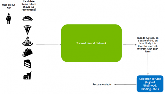
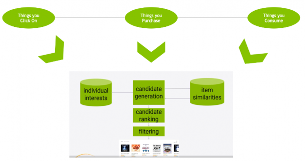
This inference stage utilizes a different pattern of data consumption than during training:
- Candidate generation: pair a user with hundreds or thousands of candidate items based on learned user-item similarity.
- Candidate ranking: rank the likelihood that the user enjoys each item.
- Filter: show the user the item they are rated most likely to enjoy.
Deep Neural Network Models for Recommendation
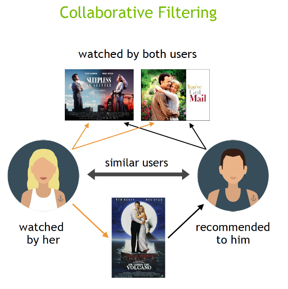
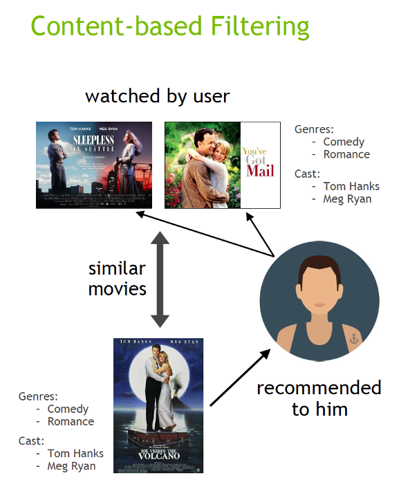
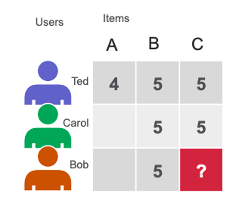
Deep learning (DL) recommender models build upon existing techniques such as factorization to model the interactions between variables and embeddings to handle categorical variables. An embedding is a learned vector of numbers representing entity features so that similar entities (users or items) have similar distances in the vector space. For example, a deep learning approach to collaborative filtering learns the user and item embeddings (latent feature vectors) based on user and item interactions with a neural network.
DL techniques also tap into the vast and rapidly growing novel network architectures and optimization algorithms to train on large amounts of data, use the power of deep learning for feature extraction, and build more expressive models. DL–based models build upon the different variations of artificial neural networks (ANNs), such as the following:
- Feedforward neural networks are ANNS where information is only fed forward from one layer to the next.
- Multilayer perceptrons (MLPs) are a type of feedforward ANN consisting of at least three layers of nodes: an input layer, a hidden layer, and an output layer. MLPs are flexible networks that can be applied to a variety of scenarios.
- Convolutional Neural Networks are the image crunchers to identify objects.
- Recurrent neural networks are the mathematical engines to parse language patterns and sequenced data.
GPUs, with their massively parallel architecture, are driving the advancement of deep learning (DL) and RecSys DL in the past several years. With GPUs, you can exploit data parallelism through columnar data processing instead of traditional row-based reading designed initially for CPUs. This provides higher performance and cost savings. Current DL–based models for recommender systems like DLRM, Wide and Deep (W&D), Neural Collaborative Filtering (NCF), Variational AutoEncoder (VAE) are part of the NVIDIA GPU-accelerated DL model portfolio that covers a wide range of network architectures and applications in many different domains beyond recommender systems, including image, text and speech analysis.
Neutral Collaborative Filtering
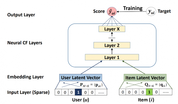
The Neural Collaborative Filtering (NCF) model is a neural network that provides collaborative filtering based on user and item interactions. The NCF model treats matrix factorization from a non-linearity perspective. NCF TensorFlow takes in a sequence of (user ID, item ID) pairs as inputs, then feeds them separately into a matrix factorization step (where the embeddings are multiplied) and into a multilayer perceptron (MLP) network.
The outputs of the matrix factorization and the MLP network are then combined and fed into a single dense layer which predicts whether the input user is likely to interact with the input item.
Variational Autoencoder for Collaborative Filtering
An autoencoder neural network reconstructs the input layer at the output layer by using the representation obtained in the hidden layer. An autoencoder for collaborative filtering learns a non-linear representation of a user-item matrix and reconstructs it by determining missing values.
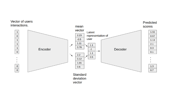
The NVIDIA GPU-accelerated Variational Autoencoder for Collaborative Filtering (VAE-CF) is an optimized implementation of the architecture first described in Variational Autoencoders for Collaborative Filtering. VAE-CF is a neural network that provides collaborative filtering based on user and item interactions. The training data for this model consists of pairs of user-item IDs for each interaction between a user and an item.
The model consists of two parts: the encoder and the decoder. The encoder is a feedforward, fully connected neural network that transforms the input vector, containing the interactions for a specific user, into an n-dimensional variational distribution. This variational distribution is used to obtain a latent feature representation of a user (or embedding). This latent representation is then fed into the decoder, which is also a feedforward network with a similar structure to the encoder. The result is a vector of item interaction probabilities for a particular user.
Wide and Deep
Wide & Deep refers to a class of networks that use the output of two parts working in parallel—wide model and deep model—whose outputs are summed to create an interaction probability. The wide model is a generalized linear model of features together with their transforms. The deep model is a Dense Neural Network (DNN), a series of hidden MLP layers, each beginning with a dense embedding of features. Categorical variables are embedded into continuous vector spaces before being fed to the DNN via learned or user-determined embeddings.
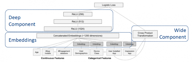
What makes this model so successful for recommendation tasks is that it provides two avenues of learning patterns in the data, “deep” and “shallow”. The complex, nonlinear DNN is capable of learning rich representations of relationships in the data and generalizing to similar items via embeddings but needs to see many examples of these relationships in order to do so well. The linear piece, on the other hand, is capable of “memorizing” simple relationships that may only occur a handful of times in the training set.
In combination, these two representation channels often end up providing more modeling power than either on its own. NVIDIA has worked with many industry partners who reported improvements in offline and online metrics by using Wide & Deep as a replacement for more traditional machine learning models.
DLRM
DLRM is a DL-based model for recommendations introduced by Facebook research. It’s designed to make use of both categorical and numerical inputs that are usually present in recommender system training data. To handle categorical data, embedding layers map each category to a dense representation before being fed into multilayer perceptrons (MLP). Numerical features can be fed directly into an MLP.
At the next level, second-order interactions of different features are computed explicitly by taking the dot product between all pairs of embedding vectors and processed dense features. Those pairwise interactions are fed into a top-level MLP to compute the likelihood of interaction between a user and item pair.
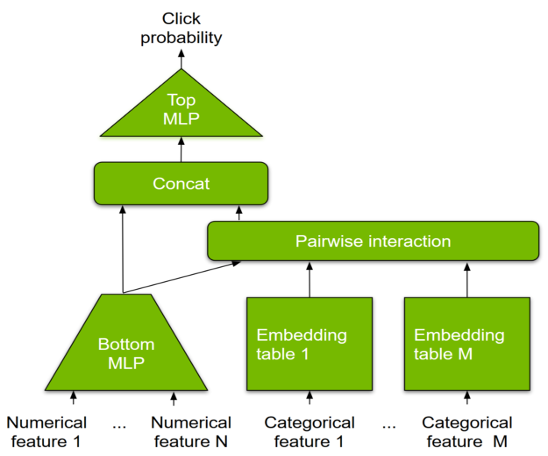
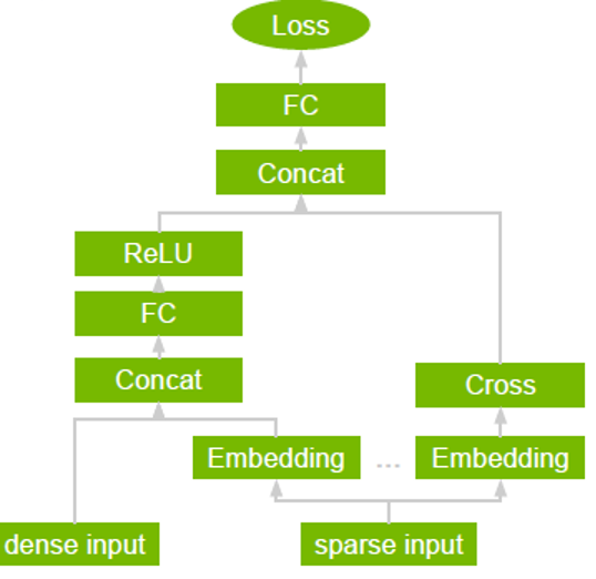
Compared to other DL-based approaches to recommendation, DLRM differs in two ways. First, it computes the feature interaction explicitly while limiting the order of interaction to pairwise interactions. Second, DLRM treats each embedded feature vector (corresponding to categorical features) as a single unit, whereas other methods (such as Deep and Cross) treat each element in the feature vector as a new unit that should yield different cross terms. These design choices help reduce computational/memory cost while maintaining competitive accuracy.
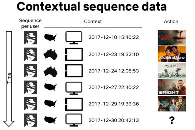
Contextual Sequence Learning
A Recurrent neural network (RNN) is a class of neural network that has memory or feedback loops that allow it to better recognize patterns in data. RNNs solve difficult tasks that deal with context and sequences, such as natural language processing, and are also used for contextual sequence recommendations. What distinguishes sequence learning from other tasks is the need to use models with an active data memory, such as LSTMs (Long Short-Term Memory) or GRU (Gated Recurrent Units) to learn temporal dependence in input data. This memory of past input is crucial for successful sequence learning. Transformer deep learning models, such as BERT (Bidirectional Encoder Representations from Transformers), are an alternative to RNNs that apply an attention technique—parsing a sentence by focusing attention on the most relevant words that come before and after it. Transformer-based deep learning models don’t require sequential data to be processed in order, allowing for much more parallelization and reduced training time on GPUs than RNNs.
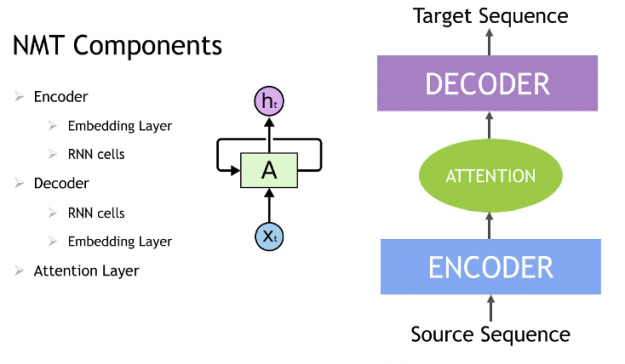
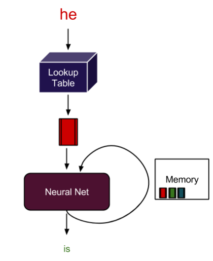
In an NLP application, input text is converted into word vectors using techniques, such as word embedding. With word embedding, each word in the sentence is translated into a set of numbers before being fed into RNN variants, Transformer, or BERT to understand context. These numbers change over time while the neural net trains itself, encoding unique properties such as the semantics and contextual information for each word, so that similar words are close to each other in this number space, and dissimilar words are far apart. These DL models provide an appropriate output for a specific language task like next-word prediction and text summarization, which are used to produce an output sequence.
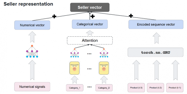
Session-based recommendations apply the advances in sequence modeling from deep learning and NLP to recommendations. RNN models train on the sequence of user events in a session (e.g. products clicked, date and time of interactions) in order to predict the probability of a user clicking the candidate or target item. User item interactions in a session are embedded similarly to words in a sentence before being fed into RNN variants such as LSTM, GRU, or Transformer to understand the context. For example, Square’s deep learning-based product recommendation system shown below leverages the transformer-based model BERT, GRUs, and NVIDIA GPUs to create a vector representation of their sellers.
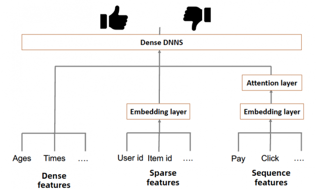
Alibaba also uses a model architecture with DNNs, GRUs and NVIDIA GPUs to support its e-commerce recommendation system which has a catalog of two billion products and can serve as many as 500 million customers per day.
In the more detailed model diagram below, you can see that GRUs are added to learn and capture the relations among the items in the user behavior sequences in order to predict if a user will click on an advertised product.
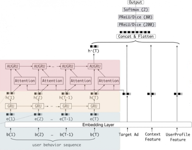
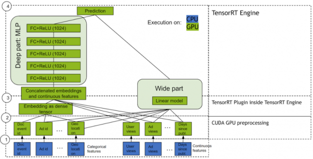
Alibaba is using thousands of T4 GPUs across its infrastructure with TensorRT to support the entire recommendation query AI pipeline on a real-time basis.
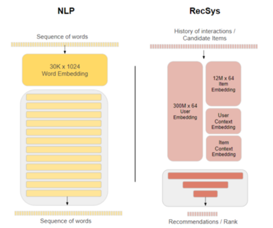
Session based recommender system architectures such as Alibaba’s Behavior Sequence Transformer follow the same general transformer architecture as for NLP, but model and embedding sizes between NLP and recommender systems vary significantly which means that you need to make sure that the entire recommendation AI pipeline is well tuned for the use case.
NVIDIA GPU Accelerated, End-to-End Data Science
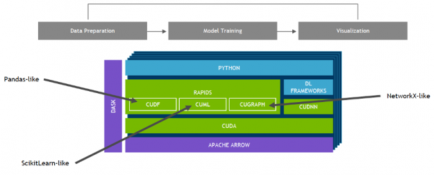
NVIDIA developed RAPIDS —an open-source data analytics and machine learning acceleration platform—for executing end-to-end data science training pipelines completely in GPUs. It relies on NVIDIA® CUDA® primitives for low-level compute optimization, but exposes that GPU parallelism and high memory bandwidth through user-friendly Python interfaces.
Focusing on common data preparation tasks for analytics and data science, RAPIDS offers a GPU-accelerated DataFrame (cuDF) that mimics the pandas API and is built on Apache Arrow. It integrates with scikit-learn and a variety of machine learning algorithms to maximize interoperability and performance without paying typical serialization costs. This allows acceleration for end-to-end pipelines—from data prep to machine learning to deep learning. RAPIDS also includes support for multi-node, multi-GPU deployments, enabling vastly accelerated processing and training on much larger dataset sizes.
Compared to similar CPU-based implementations, RAPIDS delivers 50x performance improvements for classical data analytics and machine learning (ML) processes at scale which drastically reduces the total cost of ownership (TCO) for large data science operations.
NVIDIA Merlin
NVIDIA Merlin is an open-source application framework for building high-performance, DL–based recommender systems, built on NVIDIA RAPIDS, NVIDIA CUDA® Deep Neural Network library (cuDNN), and Triton. Merlin facilitates and accelerates recommender systems on GPU, speeding up common ETL tasks, training of models, and inference serving by ~10x over commonly used methods.
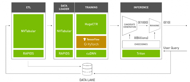
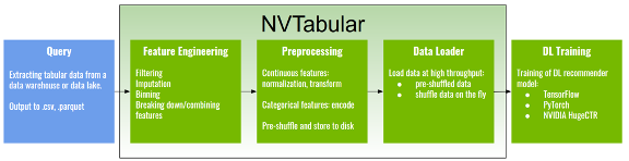
NVTabular is a feature engineering and preprocessing library for recommender systems. It provides a high-level abstraction to simplify code and accelerates computation on the GPU using the RAPIDS GPU-accelerated DataFrame cuDF library.
HugeCTR is a GPU-accelerated deep neural network training framework designed to distribute training across multiple GPUs and nodes. It supports state-of-the-art hybrid model-parallel embedding tables and data-parallel neural networks and their variants, such as Wide and Deep Learning (WDL), Deep Cross Network (DCN), DeepFM, xDeepFM, Variational Autoencoder (VAE), and Deep Learning Recommendation Model (DLRM).
NVIDIA Triton Inference Server and NVIDIA® TensorRT accelerate production inference on GPUs for feature transforms and neural network execution.
Beyond providing better performance, these libraries are also designed to be easy to use and integrate with existing recommendation pipelines.
Conclusion
In this blog, we gave an overview of deep learning models for recommender systems. Part three will discuss the NVIDIA teams’ winning solution for the ACM WSDM WebTour 21 Challenge organized by Booking.com.
Next steps
- Go to the Merlin home page
- Read:
- Introduction to NVIDIA Merlin
- Like Magic: NVIDIA Merlin Gains Adoption for Training and Inference
- Accelerated Wide and Deep Pipeline
- Building Recommender Systems Faster Using Jupyter Notebooks from NGC
- Optimizing the Deep Learning Recommendation Model on NVIDIA GPUs
- NVIDIA Merlin Accelerates Recommender Workflows with .4 Release
- Achieving High-Quality Search and Recommendation Results with DeepNLP
- NVIDIA GPUs Accelerate World’s Biggest Online Shopping Event
- Watch GTC sessions: NVIDIA Deepens Commitment to Streamlining Recommender Workflows with GTC Spring Sessions
- NVIDIA Deep Learning Institute: Building Intelligent Recommender Systems


 Google Cloud and NVIDIA collaborated to make MLOps simple, powerful, and cost-effective by bringing together the solution elements to build, serve and dynamically scale your end-to-end ML pipelines with the right-sized GPU acceleration in one place.


 Recommender systems (RecSys) have become a key component in many online services, such as e-commerce, social media, news service, or online video streaming. However with their growth in importance, the growth in scale of industry datasets, and more sophisticated models, the bar has been raised for computational resources required for recommendation systems. After NVIDIA introduced Merlin …
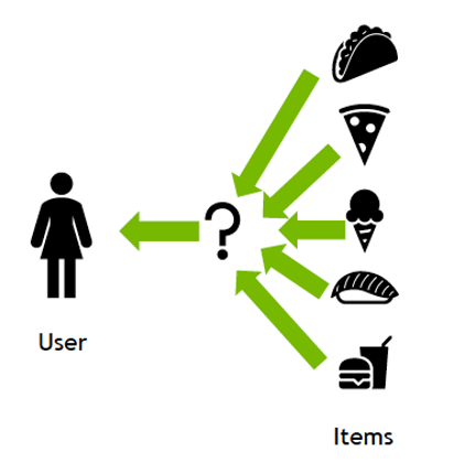

 A recent National Poetry Month feature in The Washington Post presented AI-generated artwork alongside five original poems reflecting on seasons of the past year.