Accelerating XGBoost on GPU Clusters with Dask

In XGBoost 1.0, we introduced a new, official Dask interface to support efficient distributed training.  Fast-forwarding to XGBoost 1.4, the interface is now feature-complete. If you are new to the XGBoost Dask interface, look at the first post for a gentle introduction. In this post, we look at simple code examples, showing how to maximize … Continued

In XGBoost 1.0, we introduced a new, official Dask interface to support efficient distributed training.  Fast-forwarding to XGBoost 1.4, the interface is now feature-complete. If you are new to the XGBoost Dask interface, look at the first post for a gentle introduction. In this post, we look at simple code examples, showing how to maximize the benefits of GPU acceleration.

Our examples focus on the HIGGS dataset, a moderately sized classification problem from the UCI Machine Learning repository.  In the following sections, we start from basic data loading and preprocessing with GPU-accelerated Dask and Dask-ml. Then, train an XGBoost model on returned data with different configurations. Also, share some new features along the way. After that, we showcase how to compute SHAP value on a GPU cluster and the speedup we can obtain. Lastly, we share some optimization techniques with inference.

The following examples need to be run on a machine with at least one NVIDIA GPU, which can be a laptop or a cloud instance. One of the advantages of Dask is its flexibility that users can test their code on a laptop. They can also scale up the computation to clusters with a minimum amount of code changes.  Also, to set up the environment we need xgboost==1.4, dask, dask-ml, dask-cuda, and dask-cudf python packages, available from RAPIDS conda channels:

conda install -c rapidsai -c conda-forge dask[complete] dask-ml dask-cuda dask-cudf xgboost=1.4.2

Loading the data with Dask on a GPU cluster

First we download the dataset into the data directory.

mkdir data
curl http://archive.ics.uci.edu/ml/machine-learning-databases/00280/HIGGS.csv.gz --output ./data/HIGGS.csv.gz

Then set up the GPU cluster using dask-cuda:

import os
from time import time
from typing import Tuple

from dask import dataframe as dd
from dask_cuda import LocalCUDACluster
from distributed import Client, wait
import dask_cudf
from dask_ml.model_selection import train_test_split

import xgboost as xgb
from xgboost import dask as dxgb
import numpy as np
import argparse

# … main content to be inserted here in the following sections

if __name__ == "__main__":
   parser = argparse.ArgumentParser()
   parser.add_argument("--n_workers", type=int, required=True)
   args = parser.parse_args()
   with LocalCUDACluster(args.n_workers) as cluster:
       print("dashboard:", cluster.dashboard_link)
       with Client(cluster) as client:
           main(client)

Given a cluster, we start loading the data into GPUs.  Because the data is loaded multiple times during parameter tuning, we convert the CSV file into Parquet format for better performance.  This can be easily done using dask_cudf:

def to_parquet() -> str:
   """Convert the HIGGS.csv file to parquet files."""
   dirpath = "./data"
   parquet_path = os.path.join(dirpath, "HIGGS.parquet")
   if os.path.exists(parquet_path):
       return parquet_path
   csv_path = os.path.join(dirpath, "HIGGS.csv")
   colnames = ["label"] + ["feature-%02d" % i for i in range(1, 29)]
   df = dask_cudf.read_csv(csv_path, header=None, names=colnames, dtype=np.float32)
   df.to_parquet(parquet_path)
   return parquet_path

After data loading, we prepare the training/validation splits:

def load_higgs(
    path,
) -> Tuple[
    dask_cudf.DataFrame, dask_cudf.Series, dask_cudf.DataFrame, dask_cudf.Series
]:
    df = dask_cudf.read_parquet(path)

    y = df["label"]
    X = df[df.columns.difference(["label"])]

    X_train, X_valid, y_train, y_valid = train_test_split(
        X, y, test_size=0.33, random_state=42
    )
    X_train, X_valid, y_train, y_valid = client.persist(
        [X_train, X_valid, y_train, y_valid]
    )
    wait([X_train, X_valid, y_train, y_valid])

    return X_train, X_valid, y_train, y_valid

In the preceding example, we use dask-cudf for loading data from the disk, and the train_test_split function from dask-ml for splitting up the dataset.  Most of the time, the GPU backend of dask works seamlessly with utilities in dask-ml and we can accelerate the entire ML pipeline.

Training with early stopping

One of the most frequently requested features is early stopping support for the Dask interface.  In the XGBoost 1.4 release, not only can we specify the number of stopping rounds, but also develop customized early stopping strategies.  For the simplest case, providing stopping rounds to the train function enables early stopping:

def fit_model_es(client, X, y, X_valid, y_valid) -> xgb.Booster:
   early_stopping_rounds = 5
   Xy = dxgb.DaskDeviceQuantileDMatrix(client, X, y)
   Xy_valid = dxgb.DaskDMatrix(client, X_valid, y_valid)
   # train the model
   booster = dxgb.train(
       client,
       {
           "objective": "binary:logistic",
           "eval_metric": "error",
           "tree_method": "gpu_hist",
       },
       Xy,
       evals=[(Xy_valid, "Valid")],
       num_boost_round=1000,
       early_stopping_rounds=early_stopping_rounds,
   )["booster"]
   return booster

There are two things to notice in the preceding snippet.  Firstly, we specify the number of rounds to trigger early stopping for training.  XGBoost will stop the training process once the validation metric fails to improve in consecutive X rounds, where X is the number of rounds specified for early stopping.  Secondly, we use a data type called DaskDeviceQuantileDMatrix for training but DaskDMatrix for validation.  DaskDeviceQuantileDMatrix is a drop-in replacement of DaskDMatrix for GPU-based training inputs that avoids extra data copies.

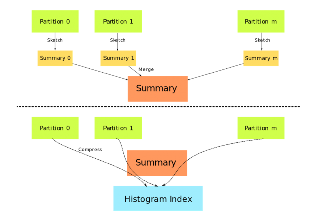
DaskDeviceQuantileDMatrix can save a considerable amount of memory when used with gpu_hist and input data is already on GPU. Figure 1 depicts the construction of DaskDeviceQuantileDMatrix.  Data partitions no longer need to be copied and concatenated, instead, a summary generated by the sketching algorithm is used as a proxy for the real data.

Inside XGBoost, early stopping is implemented as a callback function.  The new callback interface can be used to implement more advanced early stopping strategies. The following code shows an alternative implementation of early stopping, with an additional parameter asking XGBoost to return only the best model instead of the full model:

  def fit_model_customized_es(client, X, y, X_valid, y_valid):
    early_stopping_rounds = 5
    es = xgb.callback.EarlyStopping(rounds=early_stopping_rounds, save_best=True)
    Xy = dxgb.DaskDeviceQuantileDMatrix(client, X, y)
    Xy_valid = dxgb.DaskDMatrix(client, X_valid, y_valid)
    # train the model
    booster = xgb.dask.train(
        client,
        {
            "objective": "binary:logistic",
            "eval_metric": "error",
            "tree_method": "gpu_hist",
        },
        Xy,
        evals=[(Xy_valid, "Valid")],
        num_boost_round=1000,
        callbacks=[es],
    )["booster"]
    return booster

In the preceding example, the EarlyStopping callback is provided as an argument to train instead of using the early_stopping_rounds parameter. To provide a customized early stopping strategy, exploring other parameters of EarlyStopping or subclassing this callback is a great starting point.

Customized objective and evaluation metric

XGBoost is designed to be scalable through customized objective functions and metrics. In 1.4, this feature is brought to the dask interface. The requirement is exactly the same as for the single node interface:

def fit_model_customized_objective(client, X, y, X_valid, y_valid) -> dxgb.Booster:
    def logit(predt: np.ndarray, Xy: xgb.DMatrix) -> Tuple[np.ndarray, np.ndarray]:
        predt = 1.0 / (1.0 + np.exp(-predt))
        labels = Xy.get_label()
        grad = predt - labels
        hess = predt * (1.0 - predt)
        return grad, hess

    def error(predt: np.ndarray, Xy: xgb.DMatrix) -> Tuple[str, float]:
        label = Xy.get_label()
        r = np.zeros(predt.shape)
        predt = 1.0 / (1.0 + np.exp(-predt))
        gt = predt > 0.5
        r[gt] = 1 - label[gt]
        le = predt 

In the preceding function, we use the custom objective function and metric to implement a logistic regression model along with early stopping. Note that the function returns both gradient and hessian, which XGBoost uses to optimize the model.  Also, the parameter named metric_name needs to be specified in our callback. It is used to inform XGBoost that the custom error function should be used for evaluating early stopping criteria.

Explaining the model

After obtaining our first model, we might want to explain predictions using SHAP.  SHAP(SHapley Additive exPlanations) is a game theoretic approach to explain the output of machine learning models based on Shapley Value.  For details about the algorithm, please refer to the papers.  As XGBoost now has support for GPU-accelerated Shapley values, we extend this feature to the Dask interface. Now, users can compute shap values on distributed GPU clusters. This is enabled by the significantly improved predict function and the GPUTreeShap library:

def explain(client, model, X):
   # Use array instead of dataframe in case of output dim is greater than 2.
   X_array = X.values
   contribs = dxgb.predict(
       client, model, X_array, pred_contribs=True, validate_features=False
   )
   # Use the result for further analysis
   return contribs

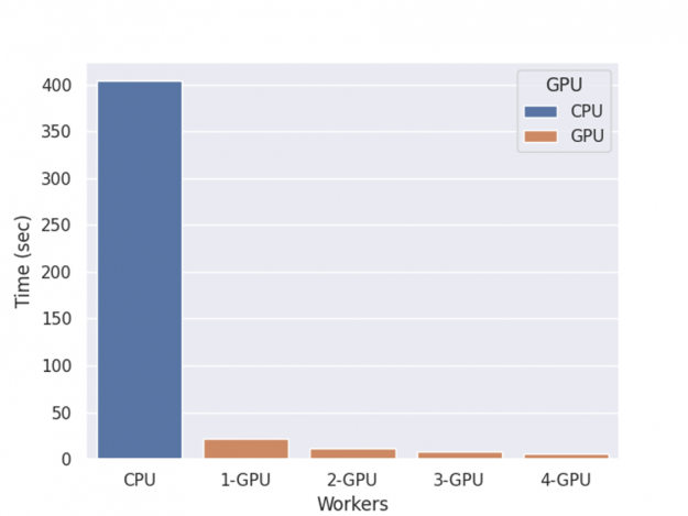
The performance of XGBoost computing shap value with multiple GPUs is shown in figure 2.

The benchmark is performed on an NVIDIA DGX-1 server with eight V100 GPUs and two 20-core Xeon E5–2698 v4 CPUs, with one round of training, shap value computation, and inference.

The resulting SHAP values can be used for visualization, tuning the column sampling with feature weights or for other data engineering purposes.

Running inference

After some tuning, we arrive at the final model for performing inference on new data. The prediction of the XGBoost Dask interface was not as efficient and also memory hungry in the older versions. In 1.4, we revised the predict function and added support for in-place prediction.  For the normal prediction, it uses the same interface with shap value computation:

def predict(client, model, X):
    predt = dxgb.predict(client, model, X)
    assert isinstance(predt, dd.Series)
    return predt

The standard predict function provides a general interface accepting both DaskDMatrix and dask collections (DataFrame or Array), but is not optimized for memory usage. Here, we replace it with in-place prediction, which supports basic inference task and doesn’t require copying the data into internal data structures of XGBoost:

def inplace_predict(client, model, X):
    # Use inplace_predict instead of standard predict.
    predt = dxgb.inplace_predict(client, model, X)
    assert isinstance(predt, dd.Series)
    return predt

The memory savings vary depending on the size of each chunk and the input types. When running inference multiple times with the same model, another potential optimization is prescattering the model. By default, XGBoost transfers the model to workers every time predict is called, incurring significant overhead. The good news is Dask functions accept a future object as a proxy to the finished model. We can then transfer data, which can overlap with other computations and persisting data on workers.

 def inplace_predict_multi_parts(client, model, X_train, X_valid):
    """Simulate the scenario that we need to run prediction on multiple datasets using train
	and valid. In real world the number of datasets is unlimited

    """
    # prescatter the model onto workers
    model_f = client.scatter(model)
    predictions = []
    for X in [X_train, X_valid]:
        # Use inplace_predict instead of standard predict.
        predt = dxgb.inplace_predict(client, model_f, X)
        assert isinstance(predt, dd.Series)
        predictions.append(predt)
        return predictions

In the preceding snippet, we pass a future model to XGBoost instead of the real one.  This way we avoid repeated transfers during prediction, or we can parallelize the model transfer with other operations like loading data, as suggested in the comments.

Putting it all together

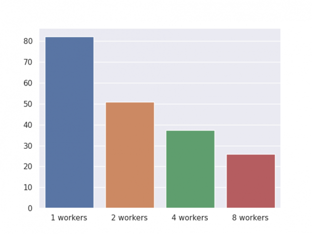
In previous sections, we demonstrate early stopping, shap value computation, customized objective, and finally inference. The following chart shows the end-to-end speed-up for a GPU cluster with varying numbers of workers.

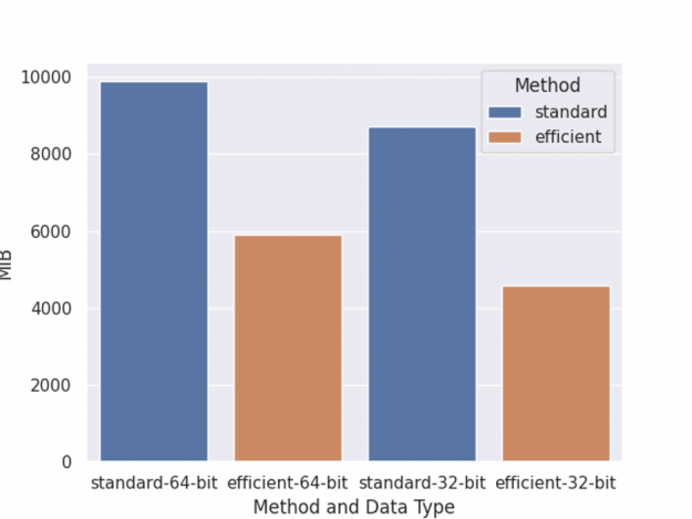
As before, the benchmark is performed on an NVIDIA DGX-1 server with eight V100 GPUs and two 20-core Xeon E5–2698 v4 CPUs, with one round of training, shap value computation, and inference. Also, we have shared two optimizations for memory usage and the overall memory usage comparison is depicted in Figure 4.

The left two columns are memory usage of training with a 64-bit data type, while the right two columns are training with a 32-bit data type. Standard means training using normal DaskDMatrix and predicts function. Efficient means using DaskDeviceQuantileDMatrix along with inplace_predict.

Scikit-learn wrapper

Previous sections consider basic model training with the ‘functional’ interface, however, there’s also a scikit-learn estimator-like interface. It’s easier to use but with some more constraints. In XGBoost 1.4, this interface has feature parity with the single node implementation. Users can choose different estimators like DaskXGBClassifier for classification and DaskXGBRanker for ranking. Check out the reference for a complete list of available estimators: https://xgboost.readthedocs.io/en/latest/python/python_api.html#module-xgboost.dask.

Summary

We have walked through an example of accelerating XGBoost on a GPU cluster with RAPIDS libraries showing that modernizing your XGBoost code can help maximize training efficiency. With the XGBoost Dask interface along with RAPIDS, users can achieve significant speedup with an easy-to-use API. Even though the XGBoost Dask interface has reached feature parity with single node API, development is continuing for better integration with other libraries for new features like hyperparameter tuning. For new feature requests relating to the dask interface, you can open an issue on XGBoost’s GitHub repository.

To learn more about using Dask and RAPIDS together, check out the NVIDIA presentations at the 2021 Dask Distributed Summit. For an overview of RAPIDS and Dask, listen into the GPU-accelerated Data Science workshop. For a deeper dive into code-based examples, check out the RAPIDS + Dask tutorial.