
|
submitted by /u/RubiksCodeNMZ [visit reddit] [comments] |
 DataBloom
|
|
submitted by /u/RubiksCodeNMZ [visit reddit] [comments] |
 The NVIDIA NGC team is hosting a webinar with live Q&A to dive into this Jupyter notebook available from the NGC catalog. Learn how to use these resources to kickstart your AI journey. Register now: NVIDIA NGC Jupyter Notebook Day: Medical Imaging Segmentation. Image segmentation partitions a digital image into multiple segments by changing the … Continued
The NVIDIA NGC team is hosting a webinar with live Q&A to dive into this Jupyter notebook available from the NGC catalog. Learn how to use these resources to kickstart your AI journey. Register now: NVIDIA NGC Jupyter Notebook Day: Medical Imaging Segmentation.
Image segmentation partitions a digital image into multiple segments by changing the representation into something more meaningful and easier to analyze. In the field of medical imaging, image segmentation can be used to help identify organs and anomalies, measure them, classify them, and even uncover diagnostic information. It does this by using data gathered from x-rays, magnetic resonance imaging (MRI), computed tomography (CT), positron emission tomography (PET), and other formats.
To achieve state-of-the-art models that deliver the desired accuracy and performance for a use case, you must set up the right environment, train with the ideal hyperparameters, and optimize it to achieve the desired accuracy. All of this can be time-consuming. Data scientists and developers need the right set of tools to quickly overcome tedious tasks. That’s why we built the NGC catalog.
The NGC catalog is a hub of GPU-optimized AI and HPC applications and tools. NGC provides easy access to performance-optimized containers, shortens model development time with pretrained models, and provides industry-specific SDKs to help build complete AI solutions and speed up AI workflows. These diverse assets can be used for a variety of use cases, ranging from computer vision and speech recognition to language understanding. The potential solutions span industries such as automotive, healthcare, manufacturing, and retail.
![NGC catalog page shows cards for GPU-optimized HPC and AI containers, pretrained models, and industry SDKs that help accelerate workflows]](https://developer-blogs.nvidia.com/wp-content/uploads/2021/07/NGC-catalog-625x381.png)
In this post, we show how you can use the Medical 3D Image Segmentation notebook to predict brain tumors in MRI images. This post is suitable for anyone who is new to AI and has a particular interest in image segmentation as it applies to medical imaging. 3D U-Net enables the seamless segmentation of 3D volumes, with high accuracy and performance. It can be adapted to solve many different segmentation problems.
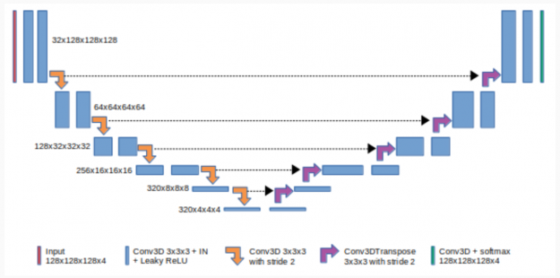
Figure 2 shows that 3D U-Net consists of a contractive (left) and expanding (right) path. It repeatedly applies unpadded convolutions followed by max pooling for downsampling.
In deep learning, a convolutional neural network (CNN) is a subset of deep neural networks, mostly used in image recognition and image processing. CNNs use deep learning to perform both generative and descriptive tasks, often using machine vision along with recommender systems and natural language processing.
Padding in CNNs refers to the number of pixels added to an image when it is processed by the kernel of a CNN. Unpadded CNNs means that no pixels are added to the image.
Pooling is a downsampling approach in CNN. Max pooling is one of common pooling methods that summarize the most activated presence of a feature. Every step in the expanding path consists of a feature map upsampling and a concatenation with the correspondingly cropped feature map from the contractive path.
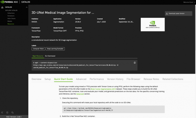
This resource contains a Dockerfile that extends the TensorFlow NGC container and encapsulates some dependencies. The resource can be downloaded using the following commands:
wget --content-disposition https://api.ngc.nvidia.com/v2/resources/nvidia/unet3d_medical_for_tensorflow/versions/20.06.0/zip -O unet3d_medical_for_tensorflow_20.06.0.zip
Aside from these dependencies, you also need the following components:
To train your model using mixed or TF32 precision with Tensor Cores or using FP32, perform the following steps using the default parameters of the 3D U-Net model on the Brain Tumor Segmentation 2019 dataset.
Download the resource manually by clicking the three dots at the top-right corner of the resource page.
You could also use the following wget command:
wget --content-disposition https://api.ngc.nvidia.com/v2/resources/nvidia/unet3d_medical_for_tensorflow/versions/20.06.0/zip -O unet3d_medical_for_tensorflow_20.06.0.zip
This command uses the Dockerfile to create a Docker image named unet3d_tf, downloading all the required components automatically.
docker build -t unet3d_tf .
Data can be obtained by registering on the Brain Tumor Segmentation 2019 dataset website. The data should be downloaded and placed where /data in the container is mounted.
To start an interactive session in the NGC container to run preprocessing, training, and inference, you must run the following command. This launches the container and mounts the ./data directory as a volume to the /data directory inside the container, mounts the ./results directory to the /results directory in the container.
The advantage of using a container is that it packages all the necessary libraries and dependencies into a single, isolated environment. This way you don’t have to worry about the complex install process.
mkdir data
mkdir results

docker run --runtime=nvidia -it --shm-size=1g --ulimit memlock=-1 --ulimit stack=67108864 --rm --ipc=host -v ${PWD}/data:/data -v ${PWD}/results:/results  -p 8888:8888 unet3d_tf:latest /bin/bash
Use this command to start a Jupyter notebook inside the container:
jupyter notebook --ip 0.0.0.0 --port 8888 --allow-root
Move the dataset to the /data directory inside the container. Download the notebook with the following command:
wget --content-disposition https://api.ngc.nvidia.com/v2/resources/nvidia/med_3dunet/versions/1/zip -O med_3dunet_1.zip
Then, upload the downloaded notebook into JupyterLab and run the cells of the notebook to preprocess the dataset and train, benchmark, and test the model.
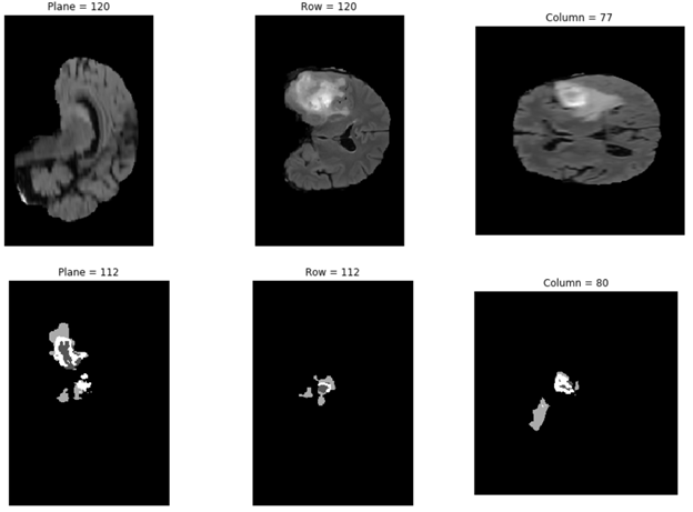
By running the cells of this Jupyter notebook, you can first check the downloaded dataset and see the brain tumor images. After that, see the data preprocessing command and prepare the data for training. The next step is training the model and using the checkpoints of the training process for the predicting step. Finally, check the output of the predict function visually.
To check the dataset, you can use nibabel, which is a package that provides read/write access to some common medical and neuroimaging file formats.
By running the next three cells, you can install nibabel using pip install, choose an image from the dataset, and plot the chosen third image from the dataset using matplotlib. You can check other dataset images by changing the image address in the code.
import nibabel as nib
import matplotlib.pyplot as plt
img_arr = nib.load('/data/MICCAI_BraTS_2019_Data_Training/HGG/BraTS19_2013_10_1/BraTS19_2013_10_1_flair.nii.gz').get_data()
def show_plane(ax, plane, cmap="gray", title=None):
ax.imshow(plane, cmap=cmap)
ax.axis("off")
if title:
ax.set_title(title)
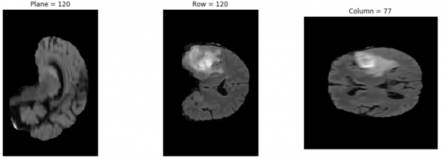
(n_plane, n_row, n_col) = img_arr.shape
_, (a, b, c) = plt.subplots(ncols=3, figsize=(15, 5))
show_plane(a, img_arr[n_plane // 2], title=f'Plane = {n_plane // 2}')
show_plane(b, img_arr[:, n_row // 2, :], title=f'Row = {n_row // 2}')
show_plane(c, img_arr[:, :, n_col // 2], title=f'Column = {n_col // 2}')
The result is something like Figure 4.
The dataset/preprocess_data.py script converts the raw data into the TFRecord format used for training and evaluation. This dataset, from the 2019 BraTS challenge, contains over 3 TB multiinstitutional, routine, clinically acquired, preoperative, multimodal, MRI scans of glioblastoma (GBM/HGG) and lower-grade glioma (LGG), with the pathologically confirmed diagnosis. When available, overall survival (OS) data for the patient is also included. This data is structured in training, validation, and testing datasets.
The format of images is nii.gz. NIfTI is a type of file format for neuroimaging. You can preprocess the downloaded dataset by running the following command:
python dataset/preprocess_data.py -i /data/MICCAI_BraTS_2019_Data_Training -o /data/preprocessed -v
The final format of the processed images is tfrecord. To help you read data efficiently, serialize your data and store it in a set of files (~100 to 200 MB each) that can each be read linearly. This is especially true if the data is being streamed over a network. It can also be useful for caching any data preprocessing. The TFRecord format is a simple format for storing a sequence of binary records, which speeds up the data loading process considerably.
After the Docker container is launched, you can start the training of a single fold (fold 0) with the default hyperparameters (for example, {1 to 8} GPUs {TF-AMP/FP32/TF32}):
Bash examples/unet3d_train_single{_TF-AMP}.sh
For example, to run with 32-bit precision (FP32 or TF32) with batch size 2 on one GPU, run the following command:
bash examples/unet3d_train_single.sh 1 /data/preprocessed /results 2
To train a single fold with mixed precision (TF-AMP) with on eight GPUs and batch size 2 per GPU, run the following command:
bash examples/unet3d_train_single_TF-AMP.sh 8 /data/preprocessed /results 2
The training performance can be evaluated by running benchmarking scripts:
bash examples/unet3d_{train,infer}_benchmark{_TF-AMP}.sh
This script makes the model run and reports the performance. For example, to benchmark training with TF-AMP with batch size 2 on four GPUs, run the following command:
bash examples/unet3d_train_benchmark_TF-AMP.sh 4 /data/preprocessed /results 2
You can use the test dataset and predict as exec-mode to test the model. The result is saved in the model_dir directory and data_dir is the path to the dataset:
python main.py --model_dir /results --exec_mode predict --data_dir /data/preprocessed_test
In the following code example, you plot one of the chosen results from the results folder:
import numpy as np
from mpl_toolkits import mplot3d
import matplotlib.pyplot as plt
data= np.load('/results/vol_0.npy')
def show_plane(ax, plane, cmap="gray", title=None):
     ax.imshow(plane, cmap=cmap)
     ax.axis("off")
     if title:
         ax.set_title(title)
(n_plane, n_row, n_col) = data.shape
_, (a, b, c) = plt.subplots(ncols=3, figsize=(15, 5))
show_plane(a, data[n_plane // 2], title=f'Plane = {n_plane // 2}')
show_plane(b, data[:, n_row // 2, :], title=f'Row = {n_row // 2}')
show_plane(c, data[:, :, n_col // 2], title=f'Column = {n_col // 2}')
For those of you looking to explore advanced features built into this notebook, you can see the full list of available options for main.py using -h or --help. By running the next cell, you can see how to change execute mode and other parameters of this script. You can perform model training, predicting, evaluating, and inferencing using customized hyperparameters using this script.
python main.py --help
The main.py parameters can be changed to perform different tasks, including training, evaluation, and prediction.
You can also train the model using default hyperparameters. By running the python main.py --help command, you can see the list of arguments that you can change, including training hyperparameters. For example, in training mode, you can change the learning rate from the default 0.0002 to 0.001 and the training steps from 16000 to 1000 using the following command:
python main.py --model_dir /results --exec_mode train --data_dir /data/preprocessed_test --learning_rate 0.001 --max_steps 1000
You can run other execution modes available in main.py. For example, in this post, we used the prediction execution mode of python.py by running the following command:
python main.py --model_dir /results --exec_mode predict --data_dir /data/preprocessed_test
In this post, we showed how you can get started with a medical imaging model using a simple Jupyter notebook from the NGC catalog. As you make the transition from this Jupyter notebook to building your own medical imaging workflows, consider using NVIDIA Clara Train. Clara Train includes AI-Assisted Annotation APIs and an Annotation server that can be seamlessly integrated into any medical viewer, making it AI-capable. The training framework includes decentralized learning techniques, such federated learning and transfer learning for your AI workflows.
To learn how to use these resources and kickstart your AI journey, register for the upcoming webinar with live Q&A, NVIDIA NGC Jupyter Notebook Day: Medical Imaging Segmentation.
Your robotaxi is arriving soon. Self-driving startup AutoX took the wraps off its full self-driving system — dubbed “Gen5” — this week. The autonomous driving platform, which is specifically designed for robotaxis, uses NVIDIA DRIVE automotive grade GPUs to reach up to 2,200 trillion operations per second (TOPS) of AI compute performance. In January, AutoX Read article >
The post AutoX Unveils Full Self-Driving System Powered by NVIDIA DRIVE appeared first on The Official NVIDIA Blog.
") Despite unprecedented progress in NLP, many state-of-the-art models are available in English only. NVIDIA has developed tools to enable the development of even the largest language models. This post describes the challenges associated with building and deploying large scale models and the solutions to enable global organizations to achieve NLP leadership in their regions.
Despite unprecedented progress in NLP, many state-of-the-art models are available in English only. NVIDIA has developed tools to enable the development of even the largest language models. This post describes the challenges associated with building and deploying large scale models and the solutions to enable global organizations to achieve NLP leadership in their regions.
Despite substantial progress in natural language processing (NLP) research over the last two years and its commercial success, little effort has been devoted to adapting this capability to other significant languages, such as Hindu, Arabic, Portuguese, or Spanish. Obviously, catering to the entire human population with more than 6,500 languages is challenging. At the same time, supporting just 40 languages addresses the NLP needs of more than 60% of the human population.
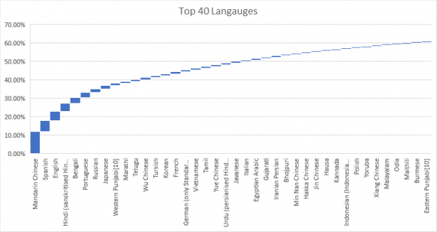
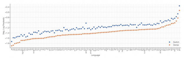
Figure 2 shows that, even across the most frequently used languages, the performance of language models varies tremendously. Bear in mind that this comparison is not perfect, as those languages do have different language entropy. More importantly, the research on most capable large-scale language models seems to be limited to only a handful of high resource languages (languages with a high number of documents available publicly), such as English or Chinese.
The situation is even more complex when you account for domain-specific languages (such as medical, technical, or legal jargon), where besides English only a few high-quality models exist. This is regretful as those domain-specific language models are currently transforming the way that clinicians, engineers, researchers or other experts access information.
Unfortunately, there is a limited number of equivalent models outside of English. Fortunately, replicating the success of English-language models across other languages is no longer a research task but predominantly an engineering activity. It no longer requires inventing new models and training approaches, but instead systematic and iterative dataset engineering, model training, and its continuous validation.
This does not mean that engineering those models is trivial. Because of the model and dataset sizes used in modern NLP, the training process requires a substantial amount of computing power. Secondly, to use large models, you must collect large textual datasets. Thirdly, because of the shared size of models used, new approaches to training and inference are required.
NVIDIA has extensive experience not only in building large-scale language models (ranging from 1 billion to 175 billion parameters) but also in deploying them to production. The goal of this post is to share our knowledge around project organization, infrastructure requirements, and budgeting and to support projects in this area.
As hypothesized in Deep Learning Scaling is Predictable, Empirically, the NLP model performance seems to follow a power law with respect to both the model size and the volume of data used for training. As you make models and datasets bigger, the performance continues to improve. The following diagram from Scaling Laws for Neural Language Models demonstrates not only that this relationship holds but more importantly, it holds across nine orders of magnitude of compute.
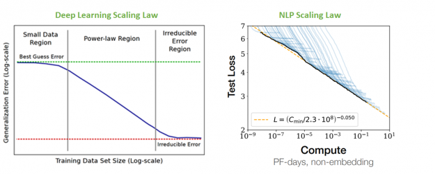
In the NLP scaling law, despite the models at the far right reaching as much as 175 billion parameters (more than 500 times larger than BERT Large), this relationship does not show signs of stopping. This suggests that even further improvement can be expected from larger models. Indeed, switch transformers when scaled to 1.6 trillion parameters (roughly 5000x larger than BERT Large) continue to demonstrate the previously mentioned behavior.
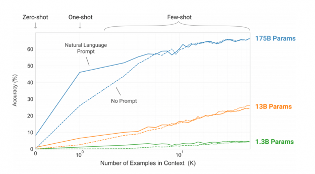
More importantly, the large NLP models seem to generate much more robust features capable of solving complex problems even without large-scale fine-tuning datasets. Figure 4 shows this capability across three orders of magnitude of models.
Due to this capability, and despite the relatively high cost of their development, large NLP models are likely to not only continue to dominate the NLP processing landscape but also continue to grow, at least by another order of magnitude approaching trillions of parameters.
This relationship between model size, dataset size, and model performance is not unique to NLP. I see the same behavior of automatic speech recognition and computer vision models, and across many other disciplines that are a backbone of conversational AI.
At the same time, a limited amount of work was devoted to the development of both large-scale datasets and models for other languages. Indeed, the majority of the work that focuses on languages other than English take advantage of smaller models and less curated datasets. For example, NLP using subset from general datasets such as raw Common Crawl).
Even less effort is devoted to supporting any of the following:
The current status creates an opportunity for local companies willing to invest in model training to lead the development of NLP technologies in the region.
Building large-scale language models is not trivial for many reasons. First, the large-scale datasets are not trivial to curate. In the raw format, they are actually quite easy to obtain. Second, the infrastructure required to train these huge models requires substantial systems knowledge to set up. Finally, they require extensive research expertise to train and optimize.
What is less widely understood is that training such large models requires software engineering effort. Most interesting models are larger than the memory capacity of not only individual GPUs but also of many multi-GPU servers. The number of mathematical operations required to train them can also make training times unmanageable, measured in months even on fairly sizable systems. Approaches such as model and pipeline parallelism overcome some of those challenges. However, applying them in a naive way could lead to scaling issues, exacerbating an already long training time.
Together with organizations such as Microsoft and Stanford University, NVIDIA has worked towards developing tools that streamline the development process of the largest language models and provide computational efficiency and scalability to allow cost-effective training. As a consequence, a wide range of tools abstracting the complexity of large model development are now available, including the following:
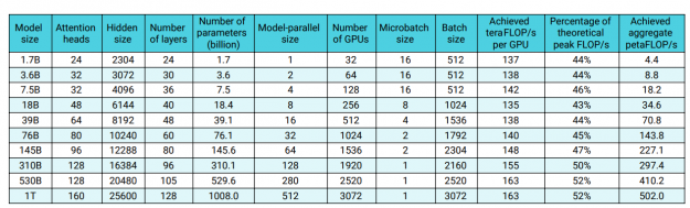
As a result of those efforts, I’ve seen a substantial reduction in training times of large models. Indeed, the GPT-3 model with 175 billion parameters trained on 300 billion tokens using 1024 NVIDIA A100 Tensor Core GPUs can be trained today in 34 days (as shown in Efficient Large-Scale Language Model Training on GPU Clusters). Based on experimentation, NVIDIA estimates that 1 trillion parameter models can be trained in approximately 84 days with 3072 A100 GPUs. Despite the training cost of those models being high, it is not beyond reach of most large organizations. With further software advances, it is likely to reduce further.
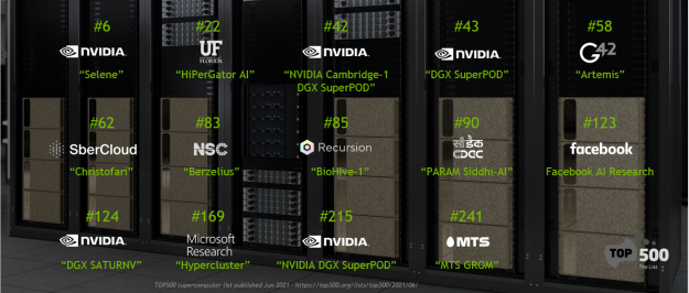
Because the development of large language models requires scalable infrastructure, NVIDIA has also consolidated knowledge from building the internal Selene cluster (used for NLP internal research and to deliver record-breaking performance in MLPerf training and inference benchmarks) into a fully packaged product called NVIDIA DGX SuperPOD. This cluster is more than just a system reference design. In fact, it can be bought in its entirety together with software and support of NVIDIA data scientists and applied researchers, similar to the NLP-focused deployment by Naver Clova).
Such an approach has already had a substantial impact on the NLP landscape, as it enables organizations with extensive NLP expertise to scale out their efforts fast. More importantly, it enables organizations with limited systems, HPC, or large-scale NLP workload expertise to start iterating in weeks, rather than months or years.
The ability to build large language models is just an academic achievement when it’s impossible to take advantage of the results of your work by deploying your models to production. The challenge of deploying models such as GPT-3 correlates to their sheer size, which exceeds the memory capacity of a GPU, and computational complexity. Both are factors that contribute to decreased throughput and high latency of inference. This is a widely understood problem and a range of tools and solutions currently exist to make serving the largest language models simple and cost-effective.
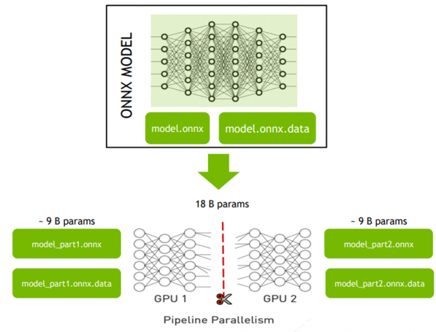
NVIDIA Triton Inference Server is an open-source cloud and edge inferencing solution optimized for both CPUs and GPUs. It can be used to host distributed models effectively. To deploy a large model using pipeline parallelism, the model must be split into several parts, for example, manipulating the ONNX graph with tools such as ONNX Graph Surgeon. Each of the parts must be small enough to fit into the memory space of a single GPU.
After the model is subdivided, it can be distributed across multiple GPUs without the need to develop any code. You create an NVIDIA Triton YAML configuration file defining how individual parts of the model should be connected.
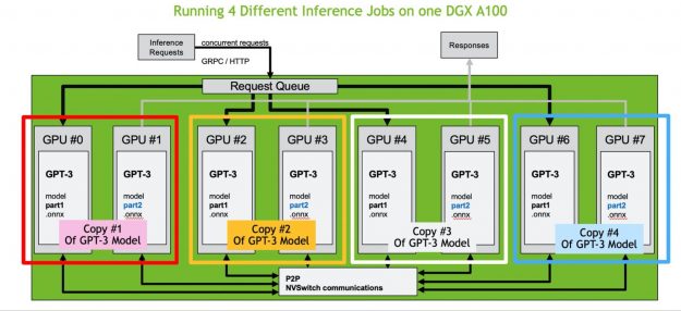
The traffic between individual model parts and their load balancing can be managed automatically by Triton Inference Server. The communication overheads are also kept to a minimum as Triton takes advantage of the latest NVIDIA NVSwitch and third-generation NVIDIA NVLink technology, providing 600 GB/sec GPU-to-GPU direct bandwidth, which is 10X higher than PCIe gen4. This means that you can efficiently deploy not only medium-scale models of multi billions of parameters but even the largest of models, including GPT-3 with trillions of parameters.
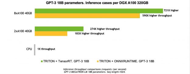
For more information, see Megatron GPT-3 Large Model Inference with Triton and ONNX Runtime (GTC21 session).
Beyond the ability to host trained large models, it is important to look at optimization techniques. Such techniques can reduce the memory footprint of the models, through quantization and pruning; substantially accelerate the execution; and reduce latency by optimizing memory access, taking advantage of TensorCores or sparsity acceleration.
Utilities such as TensorRT provide a wide range of optimized kernels for execution of transformer-based architectures. They can automatically do half precision (FP16) or, in certain cases, INT8 quantization. TensorRT also supports quantization-aware training and provides early support for hardware-accelerated sparsity.
The NVIDIA FasterTransformer library specializes in the inference of the transformer neural networks and can be used with models such as BERT or GPT-2/3. This library includes a tensor-parallel inference backend that provides the ability to do the inference of the huge GPT-3 models in parallel on multiple GPUs within the DGX A100 system. This enables you to reduce inference latency by as much as 1.2–3x, depending on model size. With FasterTransformer, you can deploy the largest of Megatron Models with a single line of code.
The Microsoft DeepSpeed library has a number of features focused on inference, including support for Mixture-of-Quantization (MoQ), high-performance INT8 kernels, or DeepFusion.
Thanks to all of those advances, large language models are no longer limited to academic research as they are making headway into commercial AI-based products.
Correct sizing of the challenge is critical for the success of your NLP initiative. The amount of engineering and research staff needed as well as training and inference infrastructure significantly affects your business case. The following factors have significant impact on the overall cost of the development:
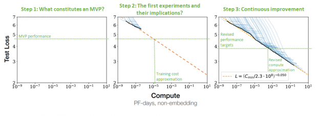
After the fundamental business questions are addressed, it is possible to estimate the effort and compute required for their development. When you have an understanding of how good your model must be to allow for the product or service, it is possible to estimate the model size needed. The relationship between the performance of language models and the amount of data and model size is widely understood (Figure 9).
After you understand the size of the model and dataset that you need, you can estimate the amount of infrastructure required and training time. For more information, see Efficient Large-Scale Language Model Training on GPU Clusters. Furthermore, the scaling of large language models is superlinear, meaning that the training performance does not degrade with the increasing model size but actually increases (Figure 10).
Here are the key factors to consider for initial infrastructure sizing:
Large language models have appealing properties and will help expand the availability of NLP around the globe. They more performant across a wide number of NLP tasks, but they are also much more sample efficient. They are what are known as few-shot learners and in certain ways are easier to design, as their exact hyperparameter configuration seems unimportant in comparison to their size. As a consequence, the NLP models are likely to continue to grow. I see empirical evidence justifying at least one if not two orders of magnitude of growth.
Fortunately, the technology to build and deploy them to production has matured considerably. The software required to train them has also matured considerably and is broadly available, such as the NVIDIA open source Megatron-based implementation of GPT-3. Quality is continuing to improve, driving down the training times. The infrastructure required to train models in this space is also well understood and commercially available (DGX SuperPOD). It is now possible to deploy the largest of NLP models to production using tools such as Triton Inference Server. As a consequence, big NLP models are in reach of everyone with the will to pursue them.
NVIDIA actively supports customers in the scoping and delivery of large training and inference systems, as well as supporting them in establishing NLP training capability. If you are working towards building your NLP capability, reach out to your local NVIDIA account team.
You can also join one of our Deep Learning Institute NLP classes. During the course, you learn how to work with modern NLP models, optimise them with TensorRT, and deploy for cost-effective production with Triton Inference Server.
For more information, see any of the following NLP-related GTC presentations:
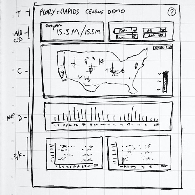
TL; DR The use of Plotly’s Dash, RAPIDS, and Data shader allows users to build viz dashboards that both render datasets of 300 million+ rows and remain highly interactive without the need for precomputed aggregations. Using RAPIDS cuDF and Plotly Dash for real-time, interactive visual analytics on GPUs Dash is an open-source framework from Plotly … Continued
TL; DR
The use of Plotly’s Dash, RAPIDS, and Data shader allows users to build viz dashboards that both render datasets of 300 million+ rows and remain highly interactive without the need for precomputed aggregations.
Dash is an open-source framework from Plotly for building interactive web application-based dashboards using Python. In addition, the RAPIDS suite of open-source software (OSS) libraries gives the freedom to execute end-to-end data science and analytics pipelines entirely on GPUs. Combining these two projects enables real-time, interactive visual analytics of multi-gigabyte datasets, even on a single GPU.
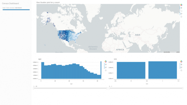
This census visualization uses the Dash API for generating charts and their callback functions. In contrast, RAPIDS cuDF is being used to accelerate these callbacks for real-time aggregations and query operations.
Using a modified version of 2010 Census data combined with 2006-2010 American Community Survey data (sourced with permission from the fantastic IPUMS.org), we mapped every individual in the United States to a single point (randomly) located onto the equivalent of a city block. As a result, each person has unique demographic attributes associated with them that enable fine-grained filtering and data discovery not previously possible. The code, installation details, and data caveats are publicly available on our GitHub.
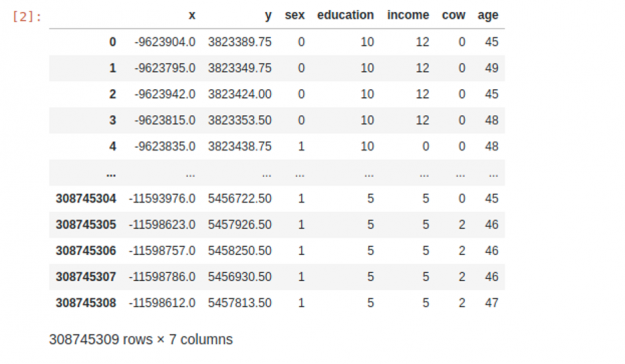
While not the most current dataset, we chose to use the 2010 Census due to its high geospatial resolution, large size, and availability. With some modification, the final dataset of 308 million rows by seven columns (type int8) was large enough to illustrate GPU acceleration’s benefits dramatically.
We decided to focus on the census dataset; the obvious choice was to search the census.gov website, which includes numerous tabulation files for download. The most applicable one, summary file 1, had a population count section with attributes that include sex, age, race, and so on. However, this dataset is tabulated to a census-block level and not to an individual level (for various privacy reasons). The result was just 211,267 rows, one for each block, with sex, age, race counts.
We chose to use the census-block boundary shapefiles to expand the row count to equal the population counts for all blocks. Then, assign a random lat-long within the boundary, and create a unique row for each person. The script to do this for each state can be found in Plotly-dash-rapids-census-demo. Switching to the more user-friendly dataset files (both SF1 and tiger boundary files) provided by the data finder tool on the IPUMS NHGIS site speeds up the process.
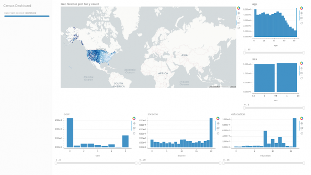
Throughout the data munging process, apart from double-checking the aggregations per block matched, we used our own cuxfilter for rapid prototyping and visual accuracy checks. In this case, it was as simple as the following snippet to have an interactive geo-scatter plot for the full 308 million rows:
Curious if we could combine additional interesting attributes to cross filter on, such as income, education, and a class of workers, we added the 5-Year 2006–2010 American Community Survey (ACS) dataset. This dataset is aggregated over census-block-groups (one level larger than census-blocks). Thus, we decided to take the aggregations over the block-groups and arbitrarily distribute them over each individual while still maintaining block-group level aggregate values. The modified dataset included:
The common column is Sex, which is used to merge all datasets. However, while this approach provides additional interesting attributes to filter on, there are a few caveats as a result:
The notebooks that execute the process can be found on plotly-dash-rapids-census-demo. The final dataset looks something like this:
Here is a quick cuxfilter dashboard to verify the dataset values:
Resource Links:
Dash supports adding individual Plotly chart objects in a dashboard, along with individual callbacks for each object figure, selection, and layout using just Python. For example, the charts in the dashboard based on the dataset above are:
This chart consists of two layers:
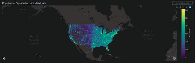
Chart update callbacks are triggered on:
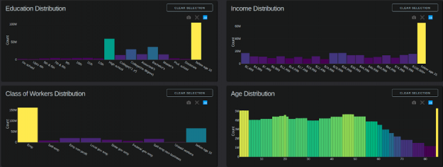
Chart update callbacks are triggered on:
Each chart in this dashboard benefits from GPU acceleration through cuDF: Using the GPU-accelerated mode, a filtering or zooming interaction generally takes around 0.2–2 seconds on a 24GB NVIDIA TITAN NVIDIA RTX. Running on a high-end CPU and 64GB of system memory, the same interaction generally takes 10–80 seconds. Typically, the cuDF GPU mode is over 20x faster than the Pandas CPU mode per chart. The 20x difference is what transforms a reporting dashboard into an interactive visual analytics application.
Though such a well-documented and usable dataset as from the Census, learning about the data and making a viz to interact with it effectively always seems to take longer than any preliminary look at the dataset might suggest.
As with all data visualization, the end result often depends on finding the appropriate balance between the data and charts you have available, the story you are trying to communicate, and the medium (and hardware) you are communicating through. For instance, we spent several iterations on column formats to ensure that the GPU usage reliably stays under our 24GB single GPU limit while still allowing for smooth interaction between multiple charts.
Working with data is complex, and working with large datasets makes it more so, but by combining Plotly Dash with RAPIDS, we accelerate the capability of analysts and data scientists. These libraries permit users to work in a familiar environment and produce bigger, faster, and more interactive visualization applications ready for production out of the box – pushing the boundaries of traditional visual analytics into the realm of high-performance computing.
Hear Josh Patterson discuss more on the RAPIDS and Plotly collaboration during the upcoming GTC Digital live webinar State of RAPIDS: Bridging the GPU Data Science Ecosystem [S22181] on May 28th at 9AM PDT.
Plotly and RAPIDS thrive from their open source communities, and we want to see them grow together. In the future, we are looking towards building tighter integration with Dash and also robust multi-GPU support with dask_cuDF.
Finally, we would like to see developers try out the tools and create awesome-looking demos on the many large-scale datasets out there, so let us know how RAPIDS made it possible to work with these datasets! Who knows, maybe we will have an even better 2020 Census visualization app ready in a year!
Plotly is also a Premier member of NVIDIA Inception, a virtual accelerator designed to support startups using GPUs for AI and data science applications. The program is open for all to apply and gives access to NVIDIA engineering support and hardware access. If interested, apply here.
This post was originally published on the RAPIDS AI blog here.
 NVIDIA EGX contains the NVIDIA GPU Operator and the new NVIDIA Network Operator 1.0 to standardize and automate the deployment of all the necessary components for provisioning Kubernetes clusters. Now released for use in production environments, the NVIDIA Network Operator makes Kubernetes networking simple and effortless for bringing AI to the enterprise.
The growing prevalence of GPU-accelerated computing in the cloud, enterprise, and at the edge increasingly relies on robust and powerful network infrastructures. NVIDIA ConnectX SmartNICs and NVIDIA BlueField DPUs provide high-throughput, low-latency connectivity that enables the scaling of GPU resources across a fleet of nodes. To address the demand for cloud-native AI workloads, NVIDIA delivers the GPU Operator, aimed at simplifying scale-out GPU deployment and management on Kubernetes.
Today, NVIDIA announced the 1.0 release of the NVIDIA Network Operator. An analog to the NVIDIA GPU Operator, the Network Operator simplifies scale-out network design for Kubernetes by automating aspects of network deployment and configuration that would otherwise require manual work. It loads the required drivers, libraries, device plugins, and CNIs on any cluster node with an NVIDIA network interface.
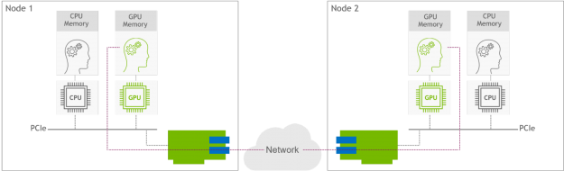
Paired with the GPU Operator, the Network Operator enables GPUDirect RDMA, a key technology that accelerates cloud-native AI workloads by orders of magnitude. The technology provides an efficient, zero-copy data transfer between NVIDIA GPUs while leveraging the hardware engines in the SmartNICs and DPUs. Figure 1 shows GPUDirect RDMA technology between two GPU nodes. The GPU on Node 1 directly communicates with the GPU on Node 2 over the network, bypassing the CPU devices.
Now available on NGC and GitHub, the NVIDIA Network Operator uses Kubernetes custom resources (CRD) and the Operator framework to provision the host software needed for enabling accelerated networking. This post discusses what’s inside the network operator, including its features and capabilities.
The Network Operator is geared towards making Kubernetes networking simple and effortless. It’s an open-source software project under the Apache 2.0 license. The 1.0 release was validated for Kubernetes running on bare-metal server infrastructure and in Linux virtualization environments. Here are the key features of the 1.0 release:
While GPU-enabled nodes are a primary use case, the Network Operator is also useful for enabling accelerated Kubernetes network environments that are independent of NVIDIA GPUs. Some examples include setting up SR-IOV networking and DPDK for accelerating telco NFV applications, establishing RDMA connectivity for fast access to NVMe storage, and more.
The Network Operator is designed from the ground up as a Kubernetes Operator that makes use of several custom resources for adding accelerated networking capabilities to a node. The 1.0 version supports several networking models adapted to both various Kubernetes networking environments and varying application requirements. Today, the Network Operator configures RoCE only for secondary networks. This means that the primary pod network remains untouched. Future work may enable configuring RoCE for the primary network.
The following sections describe the different components that are packaged and used by the Network Operator.
Node Feature Discovery (NFD) is a Kubernetes add-on for detecting hardware features and system configuration. The Network Operator uses NFD to detect nodes installed with NVIDIA SmartNICs and GPU, and label them as such. Based on those labels, the Network Operator schedules the appropriate software resources.
The Multus CNI is a container network interface (CNI) plugin for Kubernetes that enables attaching multiple network interfaces to pods. Normally in Kubernetes each Pod only has one network interface. With Multus, you can create a multihomed Pod that has multiple interfaces. Multus acting as a meta-plugin, a CNI plugin that can call multiple other CNI plugins. The NVIDIA Network Operator installs Multus to add to a container pod the secondary networks that are used for high-speed GPU-to-GPU communications.
The NVIDIA OpenFabrics Enterprise Distribution (OFED) networking libraries and drivers are packaged and tested by the NVIDIA networking team. NVIDIA OFED supports Remote Direct Memory Access (RDMA) over both Infiniband and Ethernet interconnects. The Network Operator deploys a precompiled NVIDIA OFED driver container onto each Kubernetes host using node labels. The container loads and unloads the NVIDIA OFED drivers when it is started or stopped.
The NVIDIA peer memory driver is a client that interacts with the network drivers to provide RDMA between GPUs and host memory. The Network Operator installs the NVIDIA peer memory driver on nodes that have both a ConnectX adapter and an NVIDIA GPU. This driver is also loaded and unloaded automatically when the container is started and stopped.
The Kubernetes device plugin framework advertises system hardware resources to the Kubelet agent running on a Kubernetes node. The Network Operator deploys the RDMA shared device plugin that advertises RDMA resources to Kubelet and exposes RDMA devices to Pods running on the node. It allows the Pods to perform RDMA operations. All Pods running on the node share access to the same RDMA device files.
The macvlan CNI and host-device CNI are generic container networking plugins that are hosted under the CNI project. The macvlan CNI creates a new MAC address, and forwards all traffic to the container. The host-device CNI moves an already-existing device into a container. The Network Operator uses these CNI plugins for creating macvlan networks, and assigning NIC physical functions to a container or virtual machine, respectively.
SR-IOV is a technology providing a direct interface between the virtual machine or container pod and the NIC hardware. It bypasses the host CPU and OS , frees up expensive CPU resources from I/O tasks, and greatly accelerates connectivity. The SR-IOV device plugin and CNI plugin enable advertising SR-IOV virtual functions (VFs) available on a Kubernetes node. Both are required by the Network Operator for creating and assigning SR-IOV VFs to secondary networks on which GPU-to-GPU communication is handled.
The SR-IOV Operator is designed to help the user to provision and configure the SR-IOV device plugin and SR-IOV CNI plugin in the cluster. The Network Operator uses the SR-IOV Operator to deploy and manage SR-IOV in the Kubernetes cluster.
The Whereabouts CNI is an IP address management (IPAM) CNI plugin that can assign IP addresses in a Kubernetes cluster. The Network Operator uses this CNI to assign IP addresses for secondary networks that carry GPU-to-GPU communication.
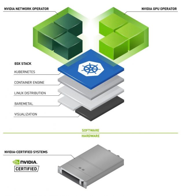
Figure 2 shows how the Network Operator works in tandem with the GPU Operator to deploy and manage the host networking software.
The following sections describe the supported networking models, and corresponding host software components.
Shared mode implies the method where a single IB device is shared between several container pods on the node. This networking model is optimized for enterprise and edge environments that require high-performance networking, without multitenancy. The Network Operator installs the following software components:
The Network Operator also installs the NVIDIA OFED Driver and NVIDIA Peer Memory on GPU nodes.
As mentioned earlier, SR-IOV is an acceleration technology that provides direct access to the NIC hardware. This networking model is optimized for multitenant Kubernetes environments, running on bare-metal. The Network Operator installs the following software components:
The Network Operator also installs the NVIDIA OFED Driver and NVIDIA Peer Memory on GPU nodes.
This networking model is suited for extremely demanding applications. The Network Operator can assign the NIC physical function to a Pod so that the Pod uses it fully. The Network Operator installs the following host software components:
The Network Operator also installs the NVIDIA OFED Driver and NVIDIA Peer Memory on GPU nodes.
The NVIDIA GPU and Network Operators are both part of the NVIDIA EGX Enterprise platform that allows GPU-accelerated computing work alongside traditional enterprise applications on the same IT infrastructure. Taken together, the operators make the NVIDIA GPU a first-class citizen in Kubernetes. Now released for use in production environments, the Network Operator streamlines Kubernetes networking, bringing the necessary levels of simplicity and scalability for enabling scale-out training and edge inferencing in the enterprise.
For more information, see the Network Operator documentation. You can also download the Network Operator from NGC to see it in action, and join the developer community in the network-operator GitHub repo.
Cybercrime cost the American public more than $4 billion in reported losses over the course of 2020, according to the FBI. To stay ahead of emerging threats, Palo Alto Networks, a global cybersecurity leader, has developed the first virtual next-generation firewall (NGFW) designed to be accelerated by NVIDIA’s BlueField data processing unit (DPU). The DPU Read article >
The post NVIDIA and Palo Alto Networks Boost Cyber Defenses with DPU Acceleration appeared first on The Official NVIDIA Blog.
 The NVIDIA Hardware Grant Program helps advance AI and data science by partnering with academic institutions around the world to enable researchers and educators with industry-leading hardware and software.
The NVIDIA Hardware Grant Program helps advance AI and data science by partnering with academic institutions around the world to enable researchers and educators with industry-leading hardware and software.
Applicants can request compute support from a large portfolio of NVIDIA products. Awardees of this highly selective program will receive a hardware donation to use in their teaching or research.
The hardware granted to qualified applicants could include NVIDIA RTX workstation GPUs powered by NVIDIA Ampere Architecture, NVIDIA BlueField Data Processing Units (DPUs), Remote V100 instances in the cloud with prebuilt container images, NVIDIA Jetson developer kits, and more. Alternatively, certain projects may be awarded with cloud compute credits instead of physical hardware.
Please note: NVIDIA RTX 30 Series GPUs are not available through the Academic Hardware Grant Program.
The current application submission window will begin on July 12 and close on July 23, 2021. The next submission window will open in early 2022.
Hi, I am looking at Tensorflow tutorials and would like some opinions on the best free Tensorflow course. I have looked at these tutorials so far:
freeCodeCamp Tensorflow complete tutorial https://youtu.be/tPYj3fFJGjk
Udacity Tensorflow tutorial https://www.udacity.com/course/intro-to-tensorflow-for-deep-learning–ud187
However, these are 1-2 years old. Do they still hold up and which of the two should I pick?
Feel free to suggest other tutorials too!
submitted by /u/Zysora
[visit reddit] [comments]

|
submitted by /u/Lazy_Acadia5970 [visit reddit] [comments] |