
|
submitted by /u/pgaleone [visit reddit] [comments] |


|
submitted by /u/pgaleone [visit reddit] [comments] |
I am trying to go through the DCGAN example on the tensorflow website https://www.tensorflow.org/tutorials/generative/dcgan. it seems to run fine up until the step where it uses the generator generated_image = generator(noise, training=False). At that point it exits with error code Process finished with exit code -1073740791 (0xC0000409).
I am running on Windows 10 using pycharm. I have tried messing with the batch size in case this is a memory issue, but even setting it to 1 gives the same results. I have also tried running pycharm as administrator.
submitted by /u/skywo1f
[visit reddit] [comments]
Hello,
I understand that Tensorflow is geared towards proprietary NVIDIA Cuda, but is there a workaround for AMD Radeon GPU? I’m on a Macbook Pro with an AMD Radeon 580 external GPU card.
submitted by /u/ZThrock
[visit reddit] [comments]


|
submitted by /u/pgaleone [visit reddit] [comments] |
I am running Tensorflow Lite on my Raspberry Pi 3b+ with a custom object detection mode. I have tested it on a Google COCO dataset and it works wonderfully but when I test it on my custom trained model it does not work despite the model passing TfLite Model Maker evaluation. When I run it the only error I get in my message is “Segmentation fault”. How can I fix this?
I am not able to upload my model to Stackoverflow but just some info about it. It is only detecting one object, It is Not quantized, it is trained based off the efficientdet_lite1 mode, and I trained it using the official Tensorflow Lite Model Maker Google Colab.
Here is the code used to interpret the model on my Pi.
I added a few print statements aswell to troubleshoot and it stops executing at around line 115.
Does anyone know how to fix this?
submitted by /u/MattDlr4
[visit reddit] [comments]
I’ve followed the same steps provided by Apple (https://developer.apple.com/metal/tensorflow-plugin/) to install the deep learning development environment on TensorFlow (based on tensorflow-metal plugin) on my MacBook Pro. My model employs the VGG19 through transfer-learning as its summary can be seen below. While I train this model on 1,859 75×75 RGB images, getting the error tensorflow.python.framework.errors_impl.InternalError: Failed copying input tensor from /job:localhost/replica:0/task:0/device:CPU:0 to /job:localhost/replica:0/task:0/device:GPU:0 in order to run _EagerConst: Dst tensor is not initialized. Isn’t this task an easy one for such a powerful SoC like M1 Pro 10-core CPU, 16-core GPU 16-core Neural Engine with 16 GB RAM? What is the issue here? Is this a bug or do I need to do some configuration to overcome this situation?
Here is the stack trace:
Metal device set to: Apple M1 Pro
systemMemory: 16.00 GB
maxCacheSize: 5.33 GB
Model: “sequential”
_________________________________________________________________
Layer (type) Output Shape Param #
=================================================================
vgg19 (Functional) (None, 512) 20024384
_________________________________________________________________
flatten (Flatten) (None, 512) 0
_________________________________________________________________
dense (Dense) (None, 1859) 953667
=================================================================
Total params: 20,978,051
Trainable params: 953,667
Non-trainable params: 20,024,384
_________________________________________________________________
Traceback (most recent call last):
File “/Users/talhakabakus/PycharmProjects/keras-matlab-comp-metal/run.py”, line 528, in <module>
run_all_stanford_dogs()
File “/Users/talhakabakus/PycharmProjects/keras-matlab-comp-metal/run.py”, line 481, in run_all_stanford_dogs
H = model.fit(X_train, y_train_cat, validation_split=n_val_split, epochs=n_epochs,
File “/Users/talhakabakus/miniforge3/envs/keras-matlab-comp-metal/lib/python3.9/site-packages/keras/engine/training.py”, line 1134, in fit
data_handler = data_adapter.get_data_handler(
File “/Users/talhakabakus/miniforge3/envs/keras-matlab-comp-metal/lib/python3.9/site-packages/keras/engine/data_adapter.py”, line 1383, in get_data_handler
return DataHandler(*args, **kwargs)
File “/Users/talhakabakus/miniforge3/envs/keras-matlab-comp-metal/lib/python3.9/site-packages/keras/engine/data_adapter.py”, line 1138, in __init__
self._adapter = adapter_cls(
File “/Users/talhakabakus/miniforge3/envs/keras-matlab-comp-metal/lib/python3.9/site-packages/keras/engine/data_adapter.py”, line 230, in __init__
x, y, sample_weights = _process_tensorlike((x, y, sample_weights))
File “/Users/talhakabakus/miniforge3/envs/keras-matlab-comp-metal/lib/python3.9/site-packages/keras/engine/data_adapter.py”, line 1031, in _process_tensorlike
inputs = tf.nest.map_structure(_convert_numpy_and_scipy, inputs)
File “/Users/talhakabakus/miniforge3/envs/keras-matlab-comp-metal/lib/python3.9/site-packages/tensorflow/python/util/nest.py”, line 869, in map_structure
structure[0], [func(*x) for x in entries],
File “/Users/talhakabakus/miniforge3/envs/keras-matlab-comp-metal/lib/python3.9/site-packages/tensorflow/python/util/nest.py”, line 869, in <listcomp>
structure[0], [func(*x) for x in entries],
File “/Users/talhakabakus/miniforge3/envs/keras-matlab-comp-metal/lib/python3.9/site-packages/keras/engine/data_adapter.py”, line 1026, in _convert_numpy_and_scipy
return tf.convert_to_tensor(x, dtype=dtype)
File “/Users/talhakabakus/miniforge3/envs/keras-matlab-comp-metal/lib/python3.9/site-packages/tensorflow/python/util/dispatch.py”, line 206, in wrapper
return target(*args, **kwargs)
File “/Users/talhakabakus/miniforge3/envs/keras-matlab-comp-metal/lib/python3.9/site-packages/tensorflow/python/framework/ops.py”, line 1430, in convert_to_tensor_v2_with_dispatch
return convert_to_tensor_v2(
File “/Users/talhakabakus/miniforge3/envs/keras-matlab-comp-metal/lib/python3.9/site-packages/tensorflow/python/framework/ops.py”, line 1436, in convert_to_tensor_v2
return convert_to_tensor(
File “/Users/talhakabakus/miniforge3/envs/keras-matlab-comp-metal/lib/python3.9/site-packages/tensorflow/python/profiler/trace.py”, line 163, in wrapped
return func(*args, **kwargs)
File “/Users/talhakabakus/miniforge3/envs/keras-matlab-comp-metal/lib/python3.9/site-packages/tensorflow/python/framework/ops.py”, line 1566, in convert_to_tensor
ret = conversion_func(value, dtype=dtype, name=name, as_ref=as_ref)
File “/Users/talhakabakus/miniforge3/envs/keras-matlab-comp-metal/lib/python3.9/site-packages/tensorflow/python/framework/tensor_conversion_registry.py”, line 52, in _default_conversion_function
return constant_op.constant(value, dtype, name=name)
File “/Users/talhakabakus/miniforge3/envs/keras-matlab-comp-metal/lib/python3.9/site-packages/tensorflow/python/framework/constant_op.py”, line 271, in constant
return _constant_impl(value, dtype, shape, name, verify_shape=False,
File “/Users/talhakabakus/miniforge3/envs/keras-matlab-comp-metal/lib/python3.9/site-packages/tensorflow/python/framework/constant_op.py”, line 283, in _constant_impl
return _constant_eager_impl(ctx, value, dtype, shape, verify_shape)
File “/Users/talhakabakus/miniforge3/envs/keras-matlab-comp-metal/lib/python3.9/site-packages/tensorflow/python/framework/constant_op.py”, line 308, in _constant_eager_impl
t = convert_to_eager_tensor(value, ctx, dtype)
File “/Users/talhakabakus/miniforge3/envs/keras-matlab-comp-metal/lib/python3.9/site-packages/tensorflow/python/framework/constant_op.py”, line 106, in convert_to_eager_tensor
return ops.EagerTensor(value, ctx.device_name, dtype)
tensorflow.python.framework.errors_impl.InternalError: Failed copying input tensor from /job:localhost/replica:0/task:0/device:CPU:0 to /job:localhost/replica:0/task:0/device:GPU:0 in order to run _EagerConst: Dst tensor is not initialized.
Process finished with exit code 1
submitted by /u/talhak
[visit reddit] [comments]
With the robotics set up we use opencv for the images. However in the cnn I use tf.io.decode_jpg to open the images. These two methods slighty alter the image and makes it such that the same image, but opened in the different methods can’t be classified on the cnn.
I found the differences in this blog: https://towardsdatascience.com/image-read-and-resize-with-opencv-tensorflow-and-pil-3e0f29b992be
which states that two things needs to be changed to ensure that the two files are the same
However the half_pixel_centers keyword is not found
https://stackoverflow.com/questions/50591669/tf-image-resize-bilinear-vs-cv2-resize
This stackoverflow states that it is added in tf2.0 with a link to their github showing it has indeed been added: https://github.com/tensorflow/tensorflow/commit/3ae2c6691b7c6e0986d97b150c9283e5cc52c15f
About my code I map the dataset to a function that reads the file path
img = tf.io.read_file(file_path)
img = tf.io.decode_jpeg(img, channels=3, dct_method=’INTEGER_ACCURATE’)
resized img = tf.image.resize(img, (28,28), method=tf.image.ResizeMethod.BILINEAR, preserve_aspect_ratio=False, antialias=False, name=None, half_pixel_center=True)
I also tried it on an other machine with tf2.7 and it gives the same error.Could someone point out what I am doing wrong or perhaps there is a better way in general?
submitted by /u/Calond
[visit reddit] [comments]
Tokenization is a fundamental pre-processing step for most natural language processing (NLP) applications. It involves splitting text into smaller units called tokens (e.g., words or word segments) in order to turn an unstructured input string into a sequence of discrete elements that is suitable for a machine learning (ML) model. ln deep learning–based models (e.g., BERT), each token is mapped to an embedding vector to be fed into the model.
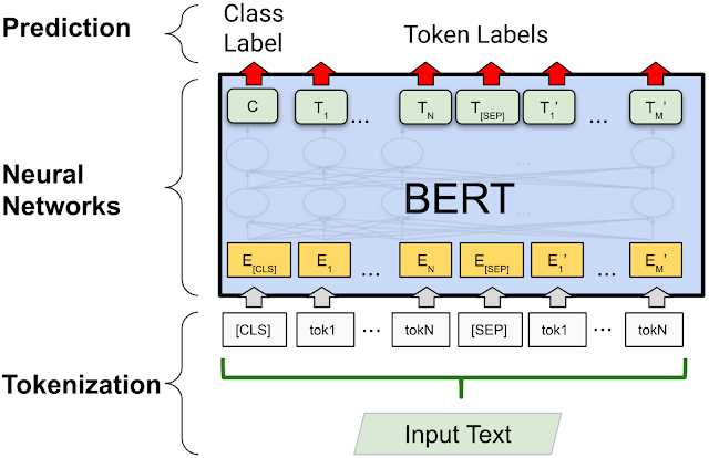 |
| Tokenization in a typical deep learning model, like BERT. |
A fundamental tokenization approach is to break text into words. However, using this approach, words that are not included in the vocabulary are treated as “unknown”. Modern NLP models address this issue by tokenizing text into subword units, which often retain linguistic meaning (e.g., morphemes). So, even though a word may be unknown to the model, individual subword tokens may retain enough information for the model to infer the meaning to some extent. One such subword tokenization technique that is commonly used and can be applied to many other NLP models is called WordPiece. Given text, WordPiece first pre-tokenizes the text into words (by splitting on punctuation and whitespaces) and then tokenizes each word into subword units, called wordpieces.
 |
| The WordPiece tokenization process with an example sentence. |
In “Fast WordPiece Tokenization”, presented at EMNLP 2021, we developed an improved end-to-end WordPiece tokenization system that speeds up the tokenization process, reducing the overall model latency and saving computing resources. In comparison to traditional algorithms that have been used for decades, this approach reduces the complexity of the computation by an order of magnitude, resulting in significantly improved performance, up to 8x faster than standard approaches. The system has been applied successfully in a number of systems at Google and has been publicly released in TensorFlow Text.
Single-Word WordPiece Tokenization
WordPiece uses a greedy longest-match-first strategy to tokenize a single word — i.e., it iteratively picks the longest prefix of the remaining text that matches a word in the model’s vocabulary. This approach is known as maximum matching or MaxMatch, and has also been used for Chinese word segmentation since the 1980s. Yet despite its wide use in NLP for decades, it is still relatively computation intensive, with the commonly adopted MaxMatch approaches’ computation being quadratic with respect to the input word length (n). This is because two pointers are needed to scan over the input: one to mark a start position, and the other to search for the longest substring matching a vocabulary token at that position.
We propose an alternative to the MaxMatch algorithm for WordPiece tokenization, called LinMaxMatch, which has a tokenization time that is strictly linear with respect to n. First, we organize the vocabulary tokens in a trie (also called a prefix tree), where each trie edge is labeled by a character, and a tree path from the root to some node represents a prefix of some token in the vocabulary. In the figure below, nodes are depicted as circles and tree edges are black solid arrows. Given a trie, a vocabulary token can be located to match an input text by traversing from the root and following the trie edges to match the input character by character; this process is referred to as trie matching.
The figure below shows the trie created from the vocabulary consisting of “a”, “abcd”, “##b”, “##bc”, and “##z”. An input text “abcd” can be matched to a vocabulary token by walking from the root (upper left) and following the trie edges with labels “a”, “b”, “c”, “d” one by one. (The leading “##” symbols are special characters used in WordPiece tokenization that are described in more detail below.)
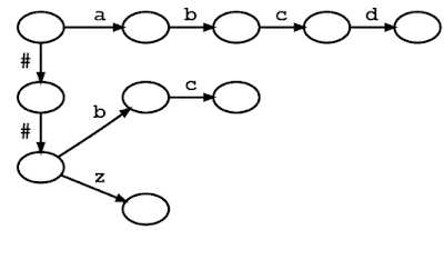 |
| Trie diagram of the vocabulary [“a”, “abcd”, “##b”, “##bc”, “##z”]. Circles and arrows represent nodes and edges along the trie, respectively. |
Second, inspired by the Aho-Corasick algorithm, a classical string-searching algorithm invented in 1975, we introduce a method that breaks out of a trie branch that fails to match the given input and skips directly to an alternative branch to continue matching. As in standard trie matching, during tokenization, we follow the trie edges to match the input characters one by one. When trie matching cannot match an input character for a given node, a standard algorithm would backtrack to the last character where a token was matched and then restart the trie matching procedure from there, which results in repetitive and wasteful iterations. Instead of backtracking, our method triggers a failure transition, which is done in two steps: (1) it collects the precomputed tokens stored at that node, which we call failure pops; and (2) it then follows the precomputed failure link to a new node from which the trie matching process continues.
For example, given a model with the vocabulary described above (“a”, “abcd”, “##b”, “##bc”, and “##z”), WordPiece tokenization distinguishes subword tokens matching at the start of the input word from the subword tokens starting in the middle (the latter being marked with two leading hashes “##”). Hence, for input text “abcz”, the expected tokenization output is [“a”, “##bc”, “##z”], where “a” matches at the beginning of the input while “##bc” and “##z” match in the middle. For this example, the figure below shows that, after successfully matching three characters ‘a’, ‘b’, ‘c’, trie matching cannot match the next character ‘z’ because “abcz” is not in the vocabulary. In this situation, LinMaxMatch conducts a failure transition by outputting the first recognized token (using the failure pop token “a”) and following the failure link to a new node to continue the matching process (in this case, node with “##bc” as the failure pop tokens).The process then repeats from the new node.
Since at least n operations are required to read the entire input, the LinMaxMatch algorithm is asymptotically optimal for the MaxMatch problem.
End-to-End WordPiece Tokenization
Whereas the existing systems pre-tokenize the input text (splitting it into words by punctuation and whitespace characters) and then call WordPiece tokenization on each resulting word, we propose an end-to-end WordPiece tokenizer that combines pre-tokenization and WordPiece into a single, linear-time pass. It uses the LinMaxMatch trie matching and failure transitions as much as possible and only checks for punctuation and whitespace characters among the relatively few input characters that are not handled by the loop. It is more efficient as it traverses the input only once, performs fewer punctuation / whitespace checks, and skips the creation of intermediate words.
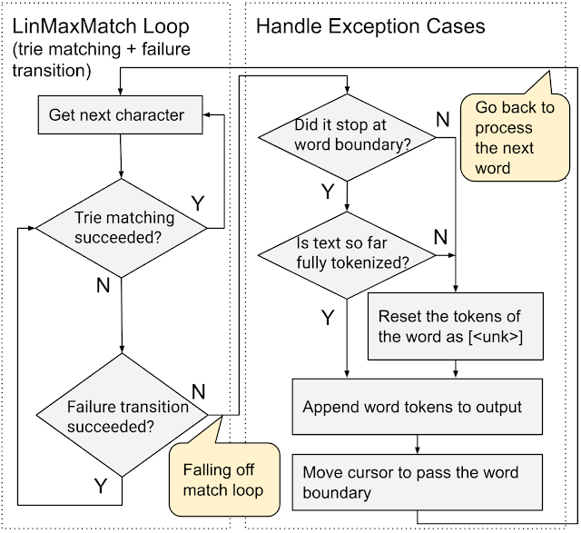 |
| End-to-End WordPiece Tokenization. |
Benchmark Results
We benchmark our method against two widely-adopted WordPiece tokenization implementations, HuggingFace Tokenizers, from the HuggingFace Transformer library, one of the most popular open-source NLP tools, and TensorFlow Text, the official library of text utilities for TensorFlow. We use the WordPiece vocabulary released with the BERT-Base, Multilingual Cased model.
We compared our algorithms with HuggingFace and TensorFlow Text on a large corpus (several million words) and found that the way the strings are split into tokens is identical to other implementations for both single-word and end-to-end tokenization.
To generate the test data, we sample 1,000 sentences from the multilingual Wikipedia dataset, covering 82 languages. On average, each word has four characters, and each sentence has 82 characters or 17 words. We found this dataset large enough because a much larger dataset (consisting of hundreds of thousands of sentences) generated similar results.
We compare the average runtime when tokenizing a single word or general text (end-to-end) for each system. Fast WordPiece tokenizer is 8.2x faster than HuggingFace and 5.1x faster than TensorFlow Text, on average, for general text end-to-end tokenization.
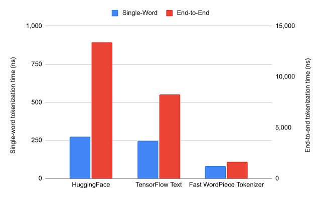 |
| Average runtime of each system. Note that for better visualization, single-word tokenization and end-to-end tokenization are shown in different scales. |
We also examine how the runtime grows with respect to the input length for single-word tokenization. Because of its linear-time complexity, the runtime of LinMaxMatch increases at most linearly with the input length, which is much slower than other quadratic-time approaches.
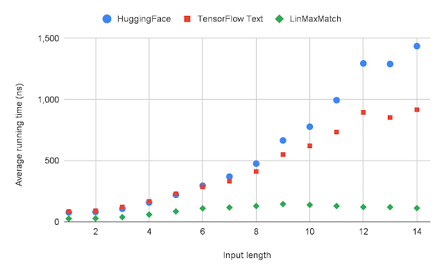 |
| The average runtime of each system with respect to the input length for single-word tokenization. |
Conclusion
We proposed LinMaxMatch for single-word WordPiece tokenization, which solves the decades-old MaxMatch problem in the asymptotically-optimal time with respect to the input length. LinMaxMatch extends the Aho-Corasick Algorithm, and the idea can be applied to more string search and transducer challenges. We also proposed an End-to-End WordPiece algorithm that combines pre-tokenization and WordPiece tokenization into a single, linear-time pass for even higher efficiency.
Acknowledgements
We gratefully acknowledge the key contributions and useful advices from other team members and colleagues, including Abbas Bazzi, Alexander Frömmgen, Alex Salcianu, Andrew Hilton, Bradley Green, Ed Chi, Chen Chen, Dave Dopson, Eric Lehman, Fangtao Li, Gabriel Schubiner, Gang Li, Greg Billock, Hong Wang, Jacob Devlin, Jayant Madhavan, JD Chen, Jifan Zhu, Jing Li, John Blitzer, Kirill Borozdin, Kristina Toutanova, Majid Hadian-Jazi, Mark Omernick, Max Gubin, Michael Fields, Michael Kwong, Namrata Godbole, Nathan Lintz, Pandu Nayak, Pew Putthividhya, Pranav Khaitan, Robby Neale, Ryan Doherty, Sameer Panwar, Sundeep Tirumalareddy, Terry Huang, Thomas Strohmann, Tim Herrmann, Tom Small, Tomer Shani, Wenwei Yu, Xiaoxue Zang, Xin Li, Yang Guo, Yang Song, Yiming Xiao, Yuan Shen, and many more.
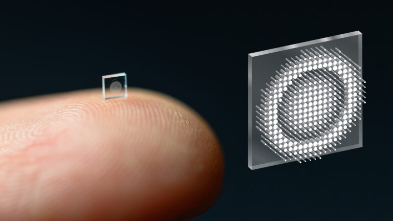 The groundbreaking technology uses an optical metasurface and machine-learning algorithms to produce high-quality color images with a wide field of view.
A team of researchers from Princeton and the University of Washington created a new camera that captures stunning images and measures in at only a half-millimeter—the size of a coarse grain of salt.
The new study, published in Nature Communications, outlines the use of optical metasurfaces with machine learning to produce high-quality color imagery, with a wide field of view. The device could be used across industries ranging from robotics to most notably the medical field, to help with disease diagnosis.
Optical metasurfaces rely on a new method of light manipulation, using cylindrical posts set on a small, square surface. The posts, which vary in geometry, work like antennas that can capture incoming photons (waves of electromagnetic radiation). These waves are then sent as signals from the metasurface to a computer to interpret and produce an image.
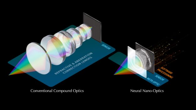
Tiny cameras offer vast potential for medical use, from brain imaging to minimally invasive endoscopies. But, up to this point, the technology has captured blurry, distorted images, with a limited field of view.
The researchers employed neural nano-optics—which combines optical metasurfaces with neural feature-based image reconstruction—to interpret the data and produce higher-quality images.
“To recover images from the measured data, we propose a feature-based deconvolution method that employs a differentiable inverse filter together with neural networks for feature extraction and refinement,” said senior author Felix Heide, an assistant professor of computer science at Princeton.
The team tested machine-learning algorithms with a simulator, comparing different configurations of the antennas. With 1.6 million cylinders on the optical surface and complex light interactions, the simulations demand massive amounts of memory.
The algorithm was tested and trained using the cuDNN-accelerated TensorFlow deep learning framework with an NVIDIA P100 GPU. The result is a new system capable of producing images comparable to a modern camera lens, from a device 500,000 times smaller. According to the study, the new camera is also 10 times better at filtering out errors than previous techniques.
“It’s been a challenge to design and configure these little microstructures to do what you want,” Ethan Tseng, a computer science Ph.D. student at Princeton and study co-lead said in a press release. “For this specific task of capturing large field of view RGB images, it’s challenging because there are millions of these little microstructures, and it’s not clear how to design them in an optimal way.”
The team is now working to add more computational abilities to the camera and envisions features such as object detection and sensors for medicine or robotics in future iterations. Beyond that, they see a use case where ultra-compact imagers turn surfaces into sensors.
“We could turn individual surfaces into cameras that have ultra-high resolution. So you wouldn’t need three cameras on the back of your phone anymore, but the whole back of your phone would become one giant camera. We can think of completely different ways to build devices in the future,” said Heide.
The raw capture data and code used to design and evaluate the neural nano-optic is publicly accessible. More information is also available on the Neural Nano-Optics for High-quality Thin Lens Imaging webpage.
Read the published research in Nature Communications. >>
Read the press release. >>
Feature image courtesy of Princeton/Ethan Tseng, et al.
Large language models (e.g., GPT-3) have many significant capabilities, such as performing few-shot learning across a wide array of tasks, including reading comprehension and question answering with very few or no training examples. While these models can perform better by simply using more parameters, training and serving these large models can be very computationally intensive. Is it possible to train and use these models more efficiently?
In pursuit of that question, today we introduce the Generalist Language Model (GLaM), a trillion weight model that can be trained and served efficiently (in terms of computation and energy use) thanks to sparsity, and achieves competitive performance on multiple few-shot learning tasks. GLaM’s performance compares favorably to a dense language model, GPT-3 (175B) with significantly improved learning efficiency across 29 public NLP benchmarks in seven categories, spanning language completion, open-domain question answering, and natural language inference tasks.
Dataset
To build GLaM, we began by building a high-quality 1.6 trillion token dataset containing language usage representative of a wide range of downstream use-cases for the model. Web pages constitute the vast quantity of data in this unlabelled corpus, but their quality ranges from professional writing to low-quality comment and forum pages. We then developed a text quality filter that was trained on a collection of text from Wikipedia and books (both of which are generally higher quality sources) to determine the quality of the content for a webpage. Finally, we applied this filter to generate the final subset of webpages and combined this with books and Wikipedia to create the final training dataset.
Model and Architecture
GLaM is a mixture of experts (MoE) model, a type of model that can be thought of as having different submodels (or experts) that are each specialized for different inputs. The experts in each layer are controlled by a gating network that activates experts based on the input data. For each token (generally a word or part of a word), the gating network selects the two most appropriate experts to process the data. The full version of GLaM has 1.2T total parameters across 64 experts per MoE layer with 32 MoE layers in total, but only activates a subnetwork of 97B (8% of 1.2T) parameters per token prediction during inference.
 |
| The architecture of GLaM where each input token is dynamically routed to two selected expert networks out of 64 for prediction. |
Similar to the GShard MoE Transformer, we replace the single feedforward network (the simplest layer of an artificial neural network, “Feedforward or FFN” in the blue boxes) of every other transformer layer with a MoE layer. This MoE layer has multiple experts, each a feedforward network with identical architecture but different weight parameters. Even though this MoE layer has many more parameters, the experts are sparsely activated, meaning that for a given input token, only two experts are used, giving the model more capacity while limiting computation. During training, each MoE layer’s gating network is trained to use its input to activate the best two experts for each token, which are then used for inference. For a MoE layer of E experts, this essentially provides a collection of E×(E-1) different feedforward network combinations (instead of one as in the classic Transformer architecture), leading to more computational flexibility.
The final learned representation of a token will be the weighted combination of the outputs from the two experts. This allows different experts to activate on different types of inputs. To enable scaling to larger models, each expert within the GLaM architecture can span multiple computational devices. We use the GSPMD compiler backend to solve the challenges in scaling the experts and train several variants (based on expert size and number of experts) of this architecture to understand the scaling effects of sparsely activated language models.
Evaluation
We use a zero-shot and one-shot setting where the tasks are never seen during training. The benchmarks for evaluation include (1) cloze and completion tasks [1,2,3]; (2) Open-domain question answering [4,5,6]; (3) Winograd-style tasks [7,8]; (4) commonsense reasoning [9,10,11]; (5) in-context reading comprehension [12,13,14,15,16]; (6) the SuperGLUE tasks; and (7) natural language inference [17]. In total, there are eight natural language generation tasks (NLG) where the generated phrases are evaluated against the ground truth targets via Exact Match (EM) accuracy and F1 measure, and 21 language understanding tasks (NLU) where the prediction from several options is chosen via conditional log-likelihood. Some tasks have variants and SuperGLUE consists of multiple tasks. Both EM accuracy and F1 are scaled from 0 to 100 across all our results and averaged for the NLG score below. The NLU score is an average of accuracy and F1 scores.
Results
GLaM reduces to a basic dense Transformer-based language model architecture when each MoE layer only has one expert. In all experiments, we adopt the notation of (base dense model size) / (number of experts per MoE layer) to describe the GLaM model. For example, 1B/64E represents the architecture of a 1B parameter dense model with every other layer replaced by a 64 expert MoE layer. In the following sections, we explore GLaM’s performance and scaling properties, including baseline dense models trained on the same datasets. Compared with the recently announced Megatron-Turing model, GLaM is on-par on the seven respective tasks if using a 5% margin, while using 5x less computation during inference.
Below, we show the 1.2T-parameter sparsely activated model (GLaM) achieved higher results on average and on more tasks than the 175B-parameter dense GPT-3 model while using less computation during inference.
 |
| Average score for GLaM and GPT-3 on NLG (left) and NLU (right) tasks (higher is better). |
Below we show a summary of the performance on 29 benchmarks compared to the dense model (GPT-3, 175B). GLaM exceeds or is on-par with the performance of the dense model on almost 80% of zero-shot tasks and almost 90% of one-shot tasks.
| Evaluation | Higher (>+5%) | On-par (within 5%) | Lower (<-5%) |
| Zero-shot | 13 | 11 | 5 |
| One-shot | 14 | 10 | 5 |
Moreover, while the full version of GLaM has 1.2T total parameters, it only activates a subnetwork of 97B parameters (8% of 1.2T) per token during inference.
| GLaM (64B/64E) | GPT-3 (175B) | |
| Total Parameters | 1.162T | 0.175T |
| Activated Parameters | 0.097T | 0.175T |
Scaling Behavior
GLaM has two ways to scale: 1) scale the number of experts per layer, where each expert is hosted within one computation device, or 2) scale the size of each expert to go beyond the limit of a single device. To evaluate the scaling properties, we compare the respective dense model (FFN layers instead of MoE layers) of similar FLOPS per token at inference time.
 |
| Average zero-shot and one-shot performance by increasing the size of each expert. The FLOPS per token prediction at inference time increases as the expert size grows. |
As shown above, performance across tasks scales with the size of the experts. GLaM sparsely activated models also perform better than dense models for similar FLOPs during inference for generation tasks. For understanding tasks, we observed that they perform similarly at smaller scales, but sparsely activated models outperform at larger scales.
Data Efficiency
Training large language models is computationally intensive, so efficiency improvements are useful to reduce energy consumption.
Below we show the computation costs for the full version of GLaM.
 |
| Computation cost in GFLOPS both for inference, per token (left) and for training (right). |
These compute costs show that GLaM uses more computation during training since it trains on more tokens, but uses significantly less computation during inference. We show comparisons using different numbers of tokens to train below.
We also evaluated the learning curves of our models compared to the dense baseline.
 |
| Average zero-shot and one-shot performance of sparsely-activated and dense models on eight generative tasks as more tokens are processed in training. |
 |
| Average zero-shot and one-shot performance of sparsely-activated and dense models on 21 understanding tasks as more tokens are processed in training. |
The results above show that sparsely activated models need to train with significantly less data than dense models to reach similar zero-shot and one-shot performance, and if the same amount of data is used, sparsely activated models perform significantly better.
Finally, we assessed the energy efficiency of GLaM.
 |
| Comparison of power consumption during training. |
While GLaM uses more computation during training, thanks to the more efficient software implementation powered by GSPMD and the advantage of TPUv4, it uses less power to train than other models.
Conclusions
Our large-scale sparsely activated language model, GLaM, achieves competitive results on zero-shot and one-shot learning and is a more efficient model than prior monolithic dense counterparts. We also show quantitatively that a high-quality dataset is essential for large language models. We hope that our work will spark more research into compute-efficient language models.
Acknowledgements
We wish to thank Claire Cui, Zhifeng Chen, Yonghui Wu, Quoc Le, Macduff Hughes, Fernando Pereira, Zoubin Ghahramani and Jeff Dean for their support and invaluable input. Special thanks to our collaborators: Yanping Huang, Simon Tong, Yanqi Zhou, Yuanzhong Xu, Dmitry Lepikhin, Orhan Firat, Maxim Krikun, Tao Wang, Noam Shazeer, Barret Zoph, Liam Fedus, Maarten Bosma, Kun Zhang, Emma Wang, David Patterson, Zongwei Zhou, Naveen Kumar, Adams Yu, Laurent Shafey, Jonathan Shen, Ben Lee, Anmol Gulati, David So, Marie Pellat, Kevin Robinson, Kathy Meier-Hellstern, Aakanksha Chowdhery, Sharan Narang, Erica Moreira and Eric Ni for helpful discussions and inspirations; and the larger Google Research team. We would also like to thank Tom Small for the animated figure used in this post.