
submitted by /u/entity14
[visit reddit] [comments]
Month: January 2022
Deep neural networks (DNNs) provide more accurate results as the size and coverage of their training data increases. While investing in high-quality and large-scale labeled datasets is one path to model improvement, another is leveraging prior knowledge, concisely referred to as “rules” — reasoning heuristics, equations, associative logic, or constraints. Consider a common example from physics where a model is given the task of predicting the next state in a double pendulum system. While the model may learn to estimate the total energy of the system at a given point in time only from empirical data, it will frequently overestimate the energy unless also provided an equation that reflects the known physical constraints, e.g., energy conservation. The model fails to capture such well-established physical rules on its own. How could one effectively teach such rules so that DNNs absorb the relevant knowledge beyond simply learning from the data?
In “Controlling Neural Networks with Rule Representations”, published at NeurIPS 2021, we present Deep Neural Networks with Controllable Rule Representations (DeepCTRL), an approach used to provide rules for a model agnostic to data type and model architecture that can be applied to any kind of rule defined for inputs and outputs. The key advantage of DeepCTRL is that it does not require retraining to adapt the rule strength. At inference, the user can adjust rule strength based on the desired operation point of accuracy. We also propose a novel input perturbation method, which helps generalize DeepCTRL to non-differentiable constraints. In real-world domains where incorporating rules is critical — such as physics and healthcare — we demonstrate the effectiveness of DeepCTRL in teaching rules for deep learning. DeepCTRL ensures that models follow rules more closely while also providing accuracy gains at downstream tasks, thus improving reliability and user trust in the trained models. Additionally, DeepCTRL enables novel use cases, such as hypothesis testing of the rules on data samples and unsupervised adaptation based on shared rules between datasets.
The benefits of learning from rules are multifaceted:
- Rules can provide extra information for cases with minimal data, improving the test accuracy.
- A major bottleneck for widespread use of DNNs is the lack of understanding the rationale behind their reasoning and inconsistencies. By minimizing inconsistencies, rules can improve the reliability of and user trust in DNNs.
- DNNs are sensitive to slight input changes that are human-imperceptible. With rules, the impact of these changes can be minimized as the model search space is further constrained to reduce underspecification.
Learning Jointly from Rules and Tasks
The conventional approach to implementing rules incorporates them by including them in the calculation of the loss. There are three limitations of this approach that we aim to address: (i) rule strength needs to be defined before learning (thus the trained model cannot operate flexibly based on how much the data satisfies the rule); (ii) rule strength is not adaptable to target data at inference if there is any mismatch with the training setup; and (iii) the rule-based objective needs to be differentiable with respect to learnable parameters (to enable learning from labeled data).
DeepCTRL modifies canonical training by creating rule representations, coupled with data representations, which is the key to enable the rule strength to be controlled at inference time. During training, these representations are stochastically concatenated with a control parameter, indicated by α, into a single representation. The strength of the rule on the output decision can be improved by increasing the value of α. By modifying α at inference, users can control the behavior of the model to adapt to unseen data.
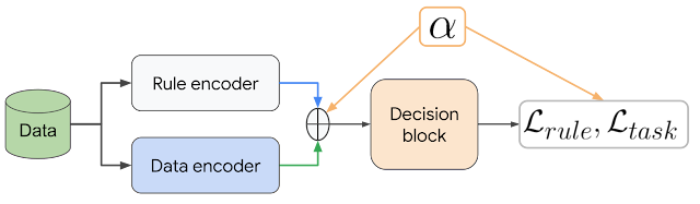 |
| DeepCTRL pairs a data encoder and rule encoder, which produce two latent representations, which are coupled with corresponding objectives. The control parameter α is adjustable at inference to control the relative weight of each encoder. |
Integrating Rules via Input Perturbations
Training with rule-based objectives requires the objectives to be differentiable with respect to the learnable parameters of the model. There are many valuable rules that are non-differentiable with respect to input. For example, “higher blood pressure than 140 is likely to lead to cardiovascular disease” is a rule that is hard to be combined with conventional DNNs. We also introduce a novel input perturbation method to generalize DeepCTRL to non-differentiable constraints by introducing small perturbations (random noise) to input features and constructing a rule-based constraint based on whether the outcome is in the desired direction.
Use Cases
We evaluate DeepCTRL on machine learning use cases from physics and healthcare, where utilization of rules is particularly important.
- Improved Reliability Given Known Principles in Physics
- Adapting to Distribution Shifts in Healthcare
We quantify reliability of a model with the verification ratio, which is the fraction of output samples that satisfy the rules. Operating at a better verification ratio could be beneficial, especially if the rules are known to be always valid, as in natural sciences. By adjusting the control parameter α, a higher rule verification ratio, and thus more reliable predictions, can be achieved.
To demonstrate this, we consider the time-series data generated from double pendulum dynamics with friction from a given initial state. We define the task as predicting the next state of the double pendulum from the current state while imposing the rule of energy conservation. To quantify how much the rule is learned, we evaluate the verification ratio.
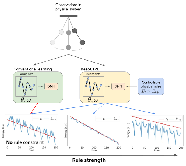 |
| DeepCTRL enables controlling a model’s behavior after learning, but without retraining. For the example of a double pendulum, conventional learning imposes no constraints to ensure the model follows physical laws, e.g., conservation of energy. The situation is similar for the case of DeepCTRL where the rule strength is low. So, the total energy of the system predicted at time t+1 ( blue) can sometimes be greater than that measured at time t (red), which is physically disallowed (bottom left). If rule strength in DeepCTRL is high, the model may follow the given rule but lose accuracy (discrepancy between red and blue is larger; bottom right). If rule strength is between the two extremes, the model may achieve higher accuracy (blue curve is close to red) and follow the rule properly (blue curve is lower than red one). |
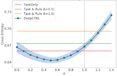
We compare the performance of DeepCTRL on this task to conventional baselines of training with a fixed rule-based constraint as a regularization term added to the objective, λ. The highest of these regularization coefficients provides the highest verification ratio (shown by the green line in the second graph below), however, the prediction error is slightly worse than that of λ = 0.1 (orange line). We find that the lowest prediction error of the fixed baseline is comparable to that of DeepCTRL, but the highest verification ratio of the fixed baseline is still lower, which implies that DeepCTRL could provide accurate predictions while following the law of energy conservation. In addition, we consider the benchmark of imposing the rule-constraint with Lagrangian Dual Framework (LDF) and demonstrate two results where its hyperparameters are chosen by the lowest mean absolute error (LDF-MAE) and the highest rule verification ratio (LDF-Ratio) on the validation set. The performance of the LDF method is highly sensitive to what the main constraint is and its output is not reliable (black and pink dashed lines).
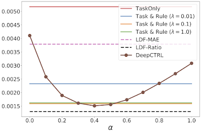 |
| Experimental results for the double pendulum task, showing the task-based mean absolute error (MAE), which measures the discrepancy between the ground truth and the model prediction, versus DeepCTRL as a function of the control parameter α. TaskOnly doesn’t have a rule constraint and Task & Rule has different rule strength (λ). LDF enforces rules by solving a constraint optimization problem. |
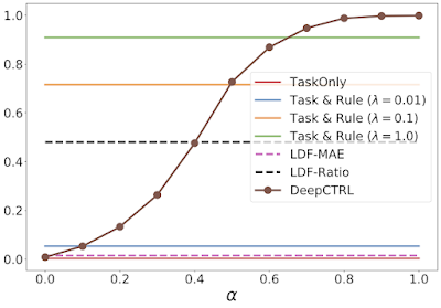 |
| As above, but showing the verification ratio from different models. |
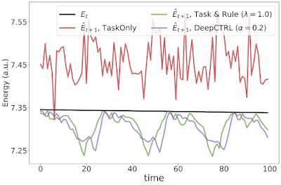 |
| Experimental results for the double pendulum task showing the current and predicted energy at time t and t + 1, respectively. |
Additionally, the figures above illustrate the advantage DeepCTRL has over conventional approaches. For example, increasing the rule strength λ from 0.1 to 1.0 improves the verification ratio (from 0.7 to 0.9), but does not improve the mean absolute error. Arbitrarily increasing λ will continue to drive the verification ratio closer to 1, but will result in worse accuracy. Thus, finding the optimal value of λ will require many training runs through the baseline model, whereas DeepCTRL can find the optimal value for the control parameter α much more quickly.
The strengths of some rules may differ between subsets of the data. For example, in disease prediction, the correlation between cardiovascular disease and higher blood pressure is stronger for older patients than younger patients. In such situations, when the task is shared but data distribution and the validity of the rule differ between datasets, DeepCTRL can adapt to the distribution shifts by controlling α.
Exploring this example, we focus on the task of predicting whether cardiovascular disease is present or not using a cardiovascular disease dataset. Given that higher systolic blood pressure is known to be strongly associated with cardiovascular disease, we consider the rule: “higher risk if the systolic blood pressure is higher”. Based on this, we split the patients into two groups: (1) unusual, where a patient has high blood pressure, but no disease or lower blood pressure, but has disease; and (2) usual, where a patient has high blood pressure and disease or low blood pressure, but no disease.
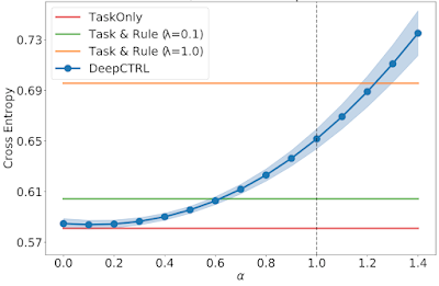
We demonstrate below that the source data do not always follow the rule, and thus the effect of incorporating the rule can depend on the source data. The test cross entropy, which indicates classification accuracy (lower cross entropy is better), vs. rule strength for source or target datasets with varying usual / unusual ratio are visualized below. The error monotonically increases as α → 1 because the enforcement of the imposed rule, which doesn’t accurately reflect the source data, becomes more strict.
 |
| Test cross entropy vs. rule strength for a source dataset with usual / unusual ratio of 0.30. |
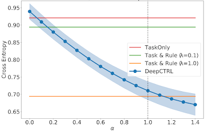
When a trained model is transferred to the target domain, the error can be reduced by controlling α. To demonstrate this, we show three domain-specific datasets, which we call Target 1, 2, and 3. In Target 1, where the majority of patients are from the usual group, as α is increased, the rule-based representation has more weight and the resultant error decreases monotonically.
 |
| As above, but for a Target dataset (1) with a usual / unusual ratio of 0.77. |
When the ratio of usual patients is decreased in Target 2 and 3, the optimal α is an intermediate value between 0 and 1. These demonstrate the capability to adapt the trained model via α.
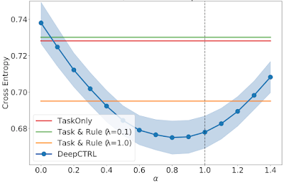 |
| As above, but for Target 2 with a usual / unusual ratio of 0.50. |
 |
| As above, but for Target 3 with a usual / unusual ratio of 0.40. |
Conclusions
Learning from rules can be crucial for constructing interpretable, robust, and reliable DNNs. We propose DeepCTRL, a new methodology used to incorporate rules into data-learned DNNs. DeepCTRL enables controllability of rule strength at inference without retraining. We propose a novel perturbation-based rule encoding method to integrate arbitrary rules into meaningful representations. We demonstrate three use cases of DeepCTRL: improving reliability given known principles, examining candidate rules, and domain adaptation using the rule strength.
Acknowledgements
We greatly appreciate the contributions of Jinsung Yoon, Xiang Zhang, Kihyuk Sohn and Tomas Pfister.

Despite the feats of modern medicine, as many as 250,000 Americans die from medical errors each year — more than 6 times the number killed in car accidents. Smart hospital AI can help avoid some of these fatalities in healthcare, just as computer vision-based driver assistance systems can improve road safety, according to AI leader Read article >
The post How Smart Hospital Technology Can Help Cut Down on Medical Errors appeared first on The Official NVIDIA Blog.
Hello, Reddit!
We currently have a decent machine learning pipeline going on but new projects/demands are coming and we’re now lacking coputational power to run everything in time. Since hardware prices skyrocketed since the begining of this pandemic, a local upgrade would be very expensive, so we’re looking for alternatives.
Can anyone suggest and comment your experience with some of these cloud GPU services? We’re running trainings 24/7 on our local machines and more “horsepower” would be appreciated. We’re looking into Paperspace Gradient, but it seems a bit of an overkill (but still cheap) and AWS.
Thanks in advance.
submitted by /u/Flashbek
[visit reddit] [comments]
Hello everyone! I have a TensorFlow Serving related question. I have also posted it to StackOverflow (https://stackoverflow.com/questions/70843006/same-model-served-via-tf-and-tf-serving-produce-different-predictions) but as no-one is answering there i thought to repost it here, maybe any of you has encountered such problems and can provide me some advice.
PROBLEM: prediction values vary in direct call and call to TF-serving (we assume the TF prediction is correct, TF-serving is incorrect)
SETUP: a TF model that uses Keras as backend and being saved as 2 files: model.h5 and architechture.json.
GOAL: predict using TF-serving
CURRENT TRIAL:
- In order to use the model on TF-serving I save the model into Saved_Model format:
model = model_from_json(json_string) model.load_weights(model_path) export_path = './gModel_Volume/3' tf.keras.models.save_model(model, export_path)
there are several approaches to save it that we tried, all produce same saved_models
-
Load the data from image is same for both setups:
X = [] X.append(preprocess_input(img_to_array(load_img(img_url_str, target_size=(260,260))))) X = np.asarray(X)
3a. for plain TF to predict we use:
#load: json_string = open(architecture_path).read() gModel = model_from_json(json_string) gModel.load_weights(model_path) #predict: predicted = gModel.predict_on_batch(X) # predicted = 0.2...
3b. for TF-servin via REST-API to predict we use:
dataToSend = X.tolist() predicted = requests.post('http://tf-serving:8501/v1/models/gModel_Volume:predict', json = {"signature_name": "serving_default", "instances": dataToSend}) # predicted = -1.17...
3c. for TF-servin via gRPC to predict we use:
GRPC_MAX_RECEIVE_MESSAGE_LENGTH = 4096 * 4096 * 3 channel = grpc.insecure_channel('tf-serving:8500', options=[('grpc.max_receive_message_length', GRPC_MAX_RECEIVE_MESSAGE_LENGTH)]) stub = prediction_service_pb2_grpc.PredictionServiceStub(channel) grpc_request = predict_pb2.PredictRequest() grpc_request.model_spec.name = 'gModel_Volume' grpc_request.model_spec.signature_name = 'serving_default' grpc_request.inputs['input_1'].CopyFrom(tf.make_tensor_proto(X)) result = stub.Predict(grpc_request,10) predicted = result.outputs['dense_1'].float_val[0] # predicted = -1.17...
As one can see the results (0.2 and -1.17) are completely different. Same saved_model was used in all cases.
Note: TF-serving is run under docker-compose and the service “tf-serving” is using the official tensorflow/serving image
I would appreciate any hits and testing suggestions.
If there are better solutions to run multiple TF models in production than TF-serving (except Cloud-based solutions like SageMaker) please share some knowledge with me.
Notes:
- Batching is disabled by default settings, but I disabled it manually too
- There are 4 different models that produce different type of output (single value, set of values, bitmap data). ALL 4 have different result while being served by TFServing and plain TF. Dimensions of the output tensors are fine, values they have are “wrong”.
submitted by /u/SG_Able
[visit reddit] [comments]
 cuFFTMp is a multi-node, multi-process extension to cuFFT that enables scientists and engineers to solve challenging problems on exascale platforms.
Today, NVIDIA announces the release of cuFFTMp for Early Access (EA). cuFFTMp is a multi-node, multi-process extension to cuFFT that enables scientists and engineers to solve challenging problems on exascale platforms.
FFTs (Fast Fourier Transforms) are widely used in a variety of fields, ranging from molecular dynamics, signal processing, computational fluid dynamics (CFD) to wireless multimedia and machine learning applications. With cuFFTMp, NVIDIA now supports not only multiple GPUs within a single system, but many GPUs across multiple nodes.
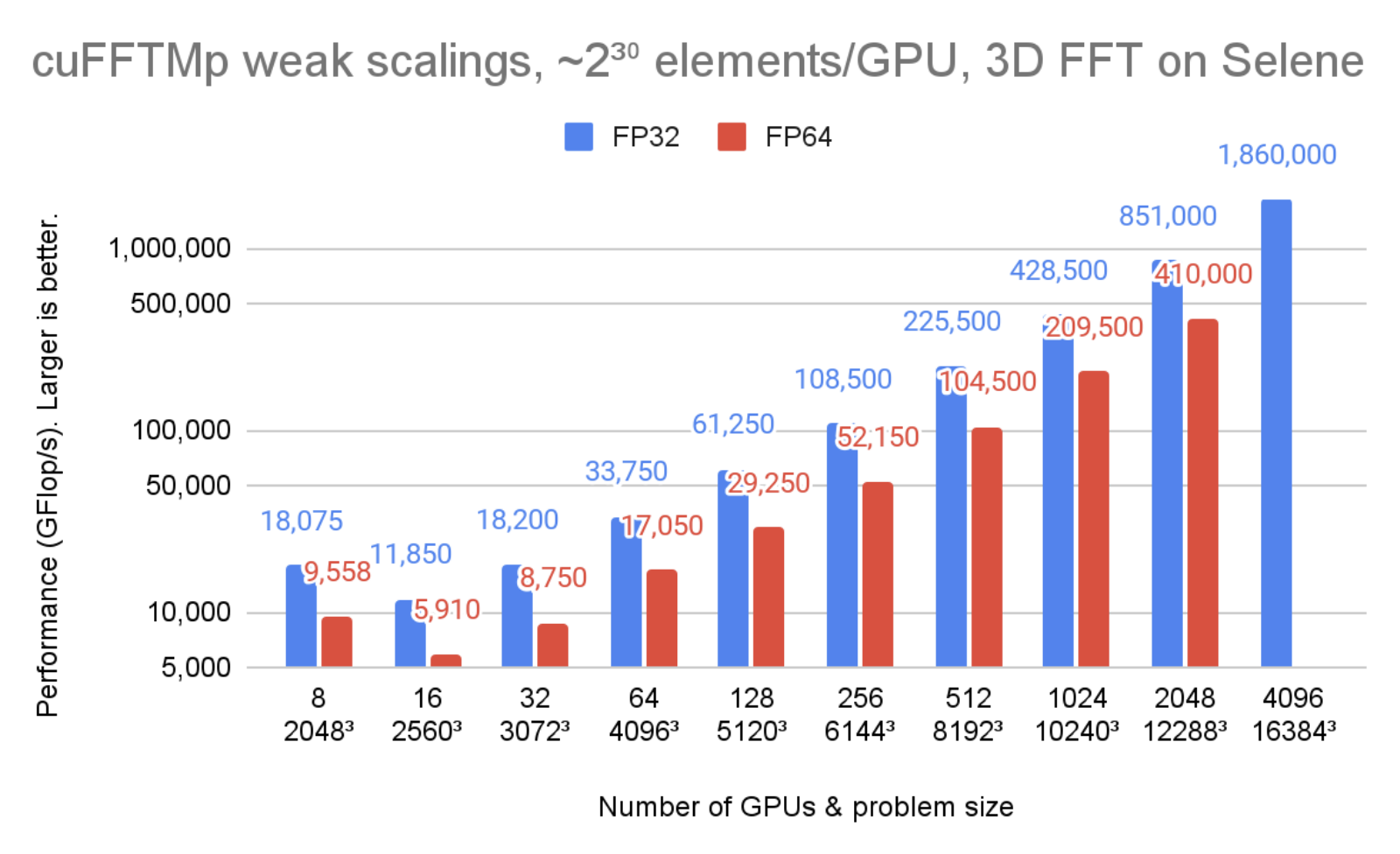
Figure 1 shows cuFFTMp reaching over 1.8 PFlop/s, more than 70% of the peak machine bandwidth for a transform of that scale.
In Figure 2, the problem size is kept unchanged but the number of GPUs is increased from 8 to 2048. You can see that cuFFTMp successfully strong-scales the problem, bringing the single-precision time from 78ms with 8 GPUs (1 node) to 4ms with 2048 GPUs (256 nodes).
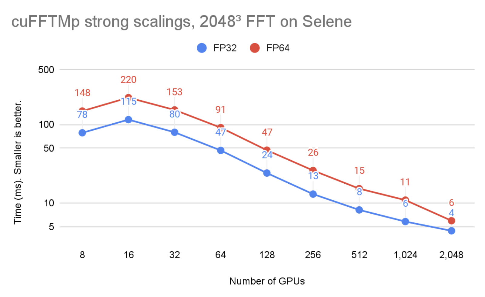
Figure 1 and 2 were run on the Selene cluster. Selene is made of NVIDIA DGXA100, 8xA100-80GB per node with NVSwitch (300 GB/s/GPU, bidirectional) and Mellanox Infiniband HDR (200 GB/s/node, bidirectional). Tests were ran using CUDA 11.4 and the NVIDIA HPC SDK 21.9 Docker container, available at nvcr.io/nvidia/nvhpc:21.9-runtime-cuda11.4-ubuntu20.04. GPU application clocks were set to the maximum.
Performance and scalability
Distributed 3D FFTs are well-known to be communication-bound because of global collective communications of the MPI_Alltoallv type. MPI_Alltoallv is the main bottleneck for distributed FFTs due to low internode bandwidth relative to high compute capabilities, and accelerator-aware MPI implementations of all_to_all type of communications vary in quality.
cuFFTMp uses NVSHMEM, a new communication library based on the OpenSHMEM standard and designed for NVIDIA GPUs by providing kernel-initiated communications. NVSHMEM creates a global address space that includes the memory of all GPUs in the cluster. Performing communication from inside CUDA kernels enables fine-grained, remote data access that reduces synchronization cost and takes advantage of the massive parallelism in the GPU to hide communication overheads.
By using NVSHMEM, cuFFTMp is independent of the quality of the MPI implementation, which is critical because performance can vary significantly from one MPI to another. For more information, see the Interim Report on Benchmarking FFT Libraries on High Performance Systems. Chapter 3.
Figure 3 shows that cuFFTMp is able to maintain roughly 75% peak as the number of GPUs are doubled.
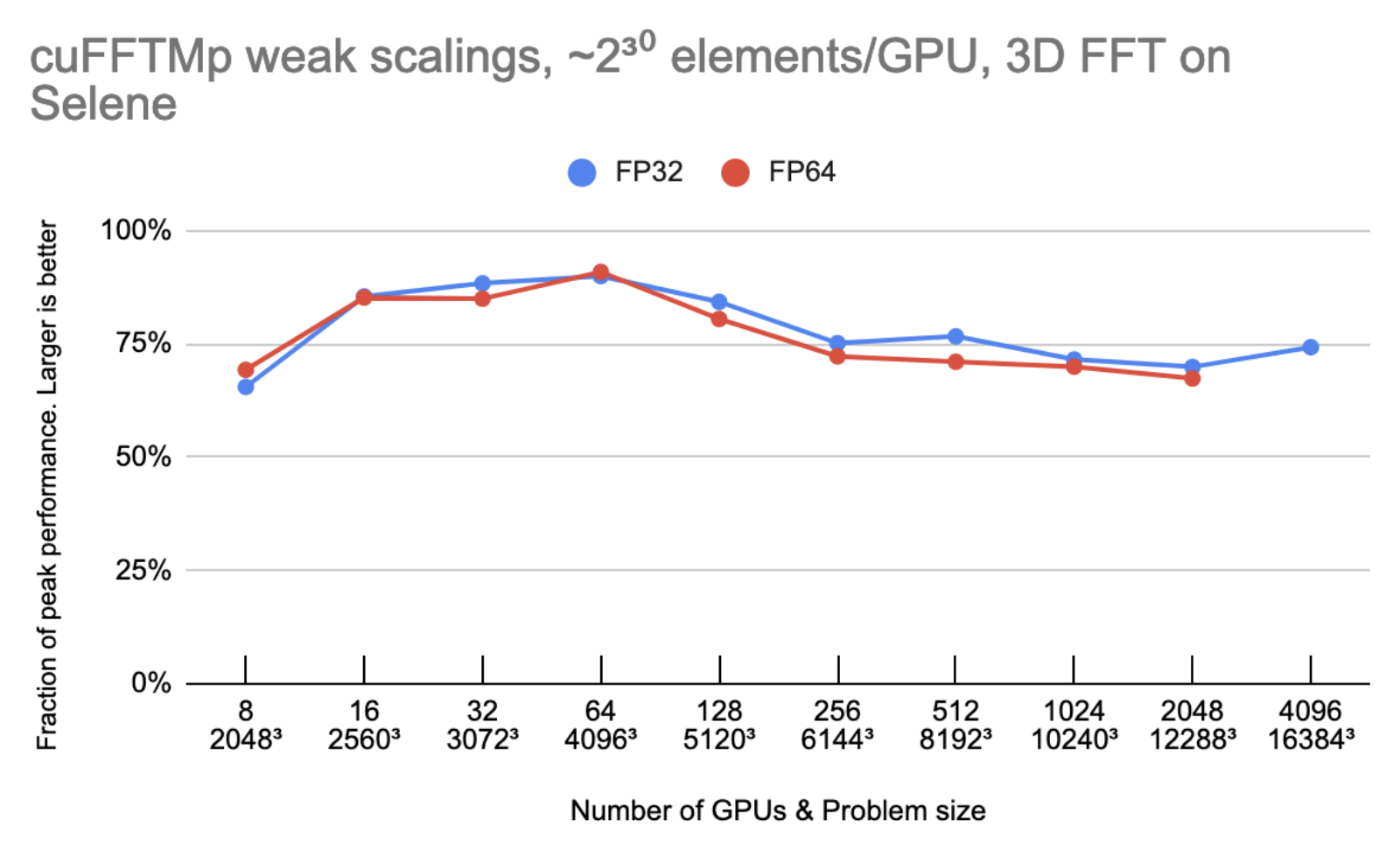
Peak performance is using 2000 GB/s/gpu for bidirectional global memory bandwidth, 300 GB/s/gpu for bidirectional NVLink bandwidth and 25 GB/s/gpu for Infiniband bandwidth.
Let N be the 1D transform size and G the number of GPUs. Every GPU owns N3/G elements (8 or 16 bytes each), and the model assumes that N3/G elements are read/written six times to or from global memory and N3/G2 elements are sent one time from every GPU to every other GPU. On 4096 GPUs, the time spent in non-InfiniBand communications accounts for less than 10% of the total time.
MPI portability and multi-architecture support
As mentioned earlier, the performances of cuFFTMp do not depend on the MPI implementation. For portability, cuFFTMp requires MPI to be launched and to manage data distributions on the CPUs.
Currently cuFFTMp statically links to NVSHMEM. NVSHMEM uses a small MPI “bootstrap plugin” (nvshmem_bootstrap_mpi.so), which is built using MPI and automatically loaded at runtime. This bootstrap targets the OpenMPI version included in the HPC SDK. For user applications that depend on another MPI implementation, the EA package includes helper scripts to build a bootstrap targeting a different MPI.
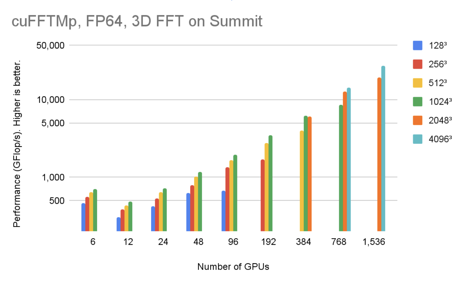
cuFFTMp supports both Linux x86_64 and IBM POWER architecture. You can download the EA package for different architectures. Figure 4 shows that, using 1536 V100 GPUs in 256 nodes, cuFFTMp can reach over 50 TFlop/s transforming 40963 complex data points with only 5% of the Summit system.
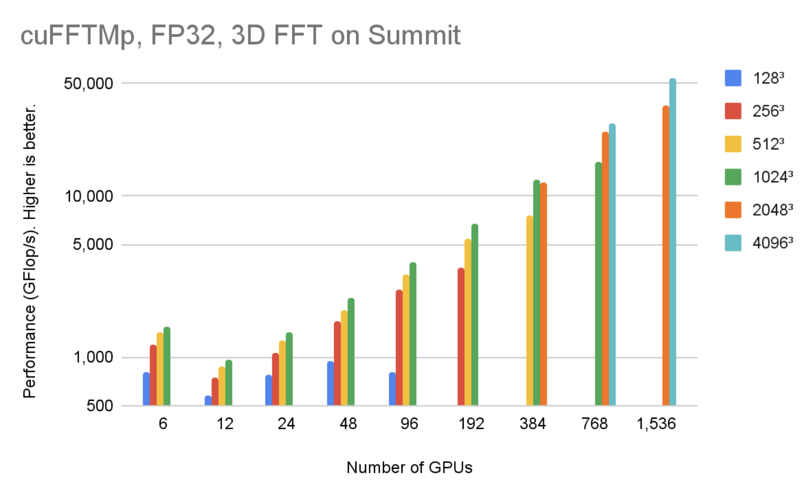
Figure 5 shows that, using 1536 V100 GPUs in 256 nodes, cuFFTMp can reach over 40 TFlop/s transforming 40963 complex data points with only 5% of the Summit system.
Easy transition to cuFFTMp
cuFFTMp is simply an extension to the current multi-GPU cuFFT library. Most existing multi-GPU functions apply to cuFFTMp. As a distributed, multiprocess library, cuFFTMp requires MPI to be bootstrapped (“launched”) and expects that data is distributed among MPI processes. The following table shows the code required to convert an application from using multi-GPU cuFFT to cuFFTMp.
| Multi-GPU, single-process cuFFT | cuFFTMp |
|---|---|
#include |
#include MPI_Init(&argc, &argv); size_t my_NX = (NX / size) + (rank size ? 1 : 0); |
| // host buffer h_f size NX*NY*NZ | // host buffer h_f size my_NX*NY*NZ |
| cufftHandle plan_c2c; cufftCreate(&plan_c2c); |
|
|
for (auto i = 0; i whichGPUs[i] = i; |
cufftMpAttachComm(plan, CUFFT_COMM_MPI, MPI_COMM_WORLD) |
|
size_t worksize; cudaLibXtDesc *d_f; cufftXtMemcpy(plan_c2c, d_f, h_f, CUFFT_COPY_HOST_TO_DEVICE); cufftXtExecDescriptor(plan_c2c, d_f, d_f, CUFFT_FORWARD) cufftXtMemcpy(plan_c2c, h_f, d_f, CUFFT_COPY_DEVICE_TO_HOST); |
|
| MPI_Finalize(); | |
Slab, pencil, and block decompositions are typical names of data distribution methods in multidimensional FFT algorithms for the purposes of parallelizing the computation across nodes. cuFFTMp EA only supports optimized slab (1D) decompositions, and provides helper functions, for example cufftXtSetDistribution and cufftMpReshape, to help users redistribute from any other data distributions to cuFFTMp’s slab data distribution.
The cuFFTMp EA package includes C++ and Fortran samples that cover a range of use cases: C2C, R2C/C2R, different plans sharing workspace, and shuffling data from one distribution to the other or redistributing across GPUs. cuFFTMp provides full support for Fortran applications, using the HPC SDK 21.7+ compilers and wrappers included in the EA package.
Customer experience: Turbulence flow simulation
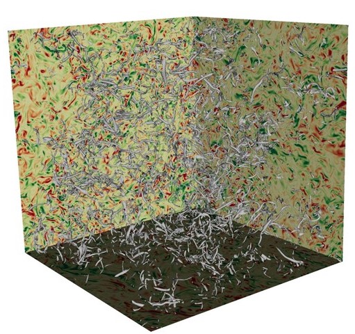
cuFFTMp enables scientists to study the challenging problem of fluid turbulence flow, the oldest unsolved problem in physics.
To understand turbulence flow behavior, a research team at the Tata Institute of Fundamental Research-Hyderabad India (TFRI) developed Fluid3D, a CFD package applying direct numerical simulation (DNS) of the Navier-Stokes equations with pseudo-spectral methods. By porting Fluid3D to cuFFTMp and CUDA, the team can now simulate higher Reynolds number flow on thousands of GPUs within a few hours, an impossible task using the MPI CPU version.
In Figure 6, turbulent flows consist of vortices of different scales, and energy is transferred from larger scales of motion to the small scales. It is important to simulate and understand the isotropic behavior of the smallest turbulent structures in large DNS runs.
DNS is a key tool to improve the understanding of turbulence flows, and pseudo-spectral methods are commonly used because of their computational efficiency and accuracy.
The challenge of turbulence flow simulation is the need to attain high Reynolds (Re) numbers. To maintain the computational stability, the Re number is limited by the grid resolution, that is, Re2.25N3, where N is the number of grid points in each dimension. Therefore, simulating high Re number turbulence flows requires numerical resolutions that can be computationally costly or even prohibitive.
Table 1 shows the grid resolutions required for the maximum Re numbers and the memory requirements for the simulations.
| Grid resolution | Simulated Reynolds number | Memory requirement (GB) |
| 10243 | 199.2 | 88 |
| 20483 | 316.2 | 704 |
| 40963 | 501.9 | 5,632 |
| 81923 | 796.8 | 45,056 |
| 122883 | 1044.1 | 152,064 |
| 163843 | 1264.8 | 360,448 |
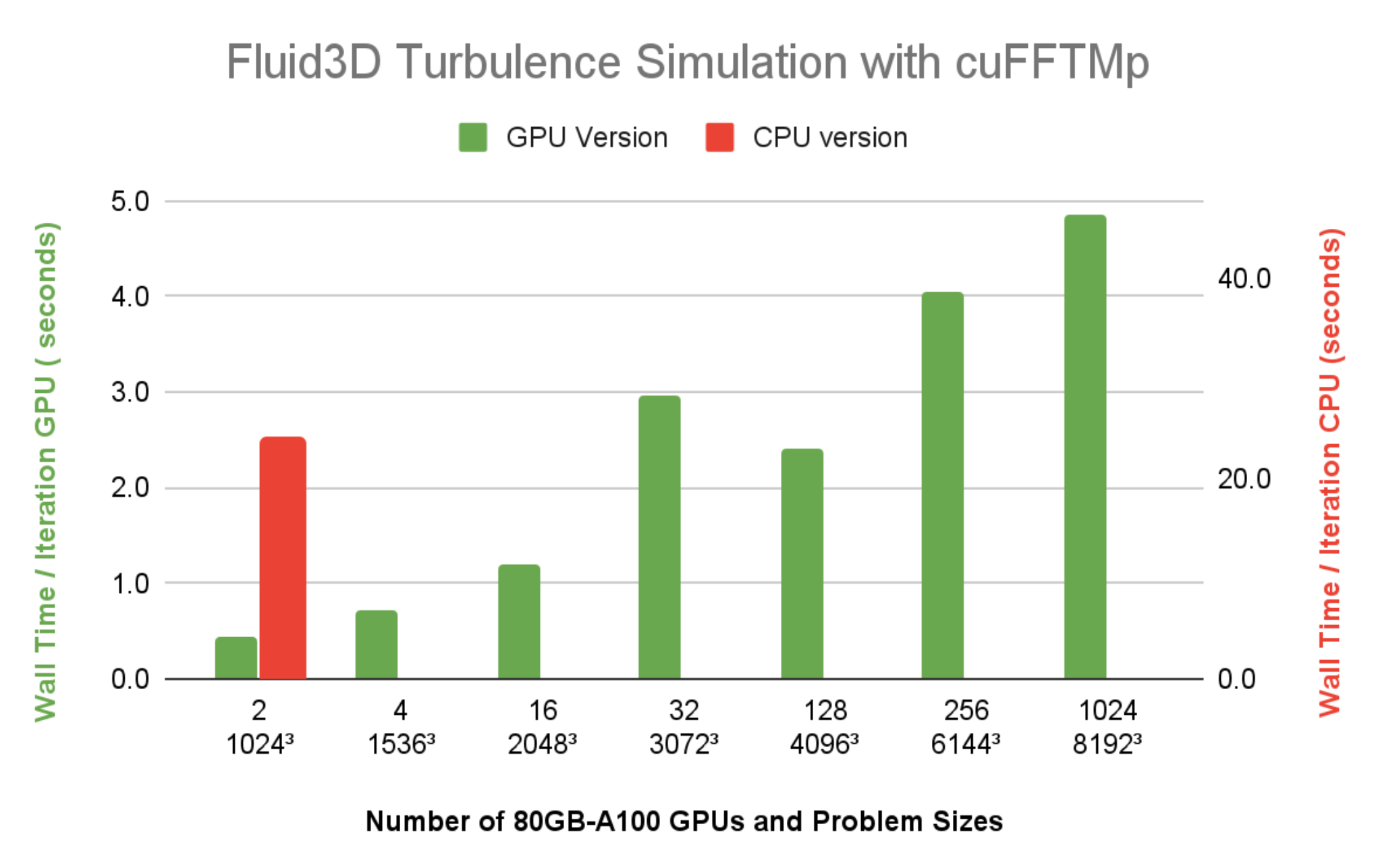
Fluid3D uses a second-order exponential Adams-Bashforth time-stepping method in the Fourier space. The simulations are typically integrated over tens of thousands of time steps, computing nine 3D-FFTs per time step. FFTs dominate the overall simulation runtime. The elapsed wall time per time step is an important metric to gauge whether the time to solution for a particular configuration of numerical experiment is reasonable.
Figure 7 shows the wall time per time step of Fluid3D is under 5 seconds, at a resolution of 81923, using 1024 A100 GPUs (128 nodes) on Selene. The CPU version with FFTW-MPI, takes 23.9 seconds per time iteration, for a resolution of 10243 problem size using 64 MPI ranks on a single 64-core CPU node. Compared to the wall time running the same 10243 problem size using two A100 GPUs, it’s clear that the speedup of Fluid3D from a CPU node to a single A100 is more than 20x.
Get started with cuFFTMp
Interested in trying out cuFFTMp to transition your application to run on multiple nodes? Head over to the Getting Started page of cuFFTMp EA. After downloading cuFFTMp, play with the sample code and see how similar they are to the multi-GPU version and how they can scale over multiple nodes.
We continue working on improving cuFFTMp, including adding batched APIs, as well as data compression to minimize communications. If you have questions or new feature requests, contact product manager Matthew Nicely.
Acknowledgments
Special thanks to Prasad Perlekar’s team at Tata Institute of Fundamental Research in Hyderabad, India, for giving us access to the multiphase turbulence flow code Fluid3D and becoming the first adopter of cuFFTMp.
We also thank the entire NVSHMEM team at NVIDIA for their help supporting the development of cuFFTMp.
 Meta’s AI supercomputer — the largest NVIDIA DGX A100 customer system to date — will deliver 5 exaflops of AI performance.
Categories
How to make custom models for tensorflow.js?
i seem to be unable to find anything about making a custom tf model for js.
so i though i’d ask here. how would you go about doing it?
whats the best way to create and train custom models, can you do it using python and use those models in js?
and if you can, then how would you do that?
also as a side note, are there any articles or video series that takes you trough this step-by-step?
thanks for all the help!
submitted by /u/CCmamo
[visit reddit] [comments]
 Nsight Compute kernel profiler now includes Range Replay, Memory Analysis, and Guided Analysis enhancements.
NVIDIA Nsight Compute is an interactive kernel profiler for CUDA applications. It provides detailed performance metrics and API debugging through a user interface and a command-line tool. Nsight Compute 2022.1 brings updates to improve data collection modes enabling new use cases and options for performance profiling.
What’s New
Range Replay
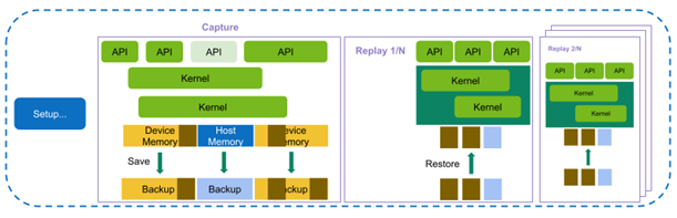
This release of Nsight Compute extends the existing replay modes with the highly requested feature of Range Replay. Range Replay captures and replays complete ranges of CUDA API calls and kernel launches within the profiled application. Metrics are associated with the entire range as opposed to individual kernels.This allows the tool to execute kernels without serialization and support profiling kernels that need to be run concurrently for correctness or performance reasons. A range consists of a start and an end marker; and includes all CUDA API calls and kernels launched between these markers from any CPU thread.
Range markers can be defined using either:
- Profiler Start/Stop API
- NVTX Ranges
For complete details, see the “Replay” section in Nsight Compute’s Kernel Profiling Guide.
Memory Analysis
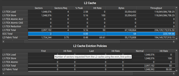
When profiling on A100, a new L2 Cache Eviction Policies table in the Memory Analysis section helps you understand the number of accesses and achieved hit rates by the various cache eviction policies. In the same section, the L2 Cache table now has a new ECC row to show traffic created from enabling hardware Error Correction Code on the GPU.
Guided Analysis
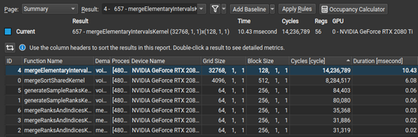
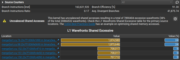
Nsight Compute now makes it easier to select initial analysis targets in multiresult collection by dynamically selecting between the Summary and Details pages when opening a report. Rules were extended to detect non-fused floating-point instructions as an optimization opportunity. Last, but not least, when the Uncoalesced Memory Access rules are triggered, they show a table of the five most valuable instances, making it easier to inspect and resolve them on the Source page.
Additional improvements
Further improvements include an Occupancy Calculator auto-update. There is also a new ‘Thread Instructions Executed’ metric and register name tooltips for the Register Dependency columns in the Source page, as well as NVLink updates.
At GTC in November of 2021, we released insightful assets showcasing Nsight tools capabilities:
- Understanding CUDA Application Behavior, Performance, and Optimization Just Got Easier with the Latest Developer Tools [A31048]
- Optimizing CUDA Machine Learning Codes with Nsight Profiling Tools [DLIT1605]
- Guided Analysis with Nsight Compute Demo
Resources
 With NVIDIA Jetson embedded platforms, teams at the DARPA SubT Challenge detected objects with both high accuracy and high throughput.
Performing real-time inference with high accuracy is a challenging task, especially in a poor-visibility environment. With NVIDIA Jetson embedded platforms, teams at the recently concluded Defense Advanced Research Projects Agency (DARPA) Subterranean (SubT) Challenge were able to detect objects of interest with both high accuracy and high throughput. In this post, we will cover the results, systems, and challenges faced by teams in the final leg of the systems competition.
The SubT Challenge is an international robotics competition organized and coordinated by DARPA. The competition encourages researchers to develop new approaches for robots to map, navigate, and search environments that pose various challenges such as poor visibility, presence of hazards, unknown maps, or poor communication infrastructure.
The challenge consists of three preliminary circuit events: Tunnel Circuit, Urban Circuit, and Cave Circuit (canceled due to the COVID-19 pandemic), as well as a final integrated challenge course. Each circuit and the final event are held in different environments with various types of terrain. According to the event organizers, the competition was held over 3 years in different phases with the final event held in September of 2021 in Louisville, KY.
Competitors in the SubT Challenge leveraged NVIDIA technology for both their hardware and software needs. Teams used desktop/server GPUs to train models that were deployed on robots using NVIDIA Jetson embedded platform for real-time detection of artifacts and objects of interest–the main criteria used to determine the winning team. Five out of seven competitors also used the Jetson platform to perform real-time object detection.
The SubT Challenge
The SubT Challenge is inspired by real-world scenarios faced by first responders during search and rescue operations or disaster response.
The state-of-the-art methods developed through this competition will help reduce the risk of casualties of search and rescue personnel and first responders while they explore the unknown underground environments. Additionally, the autonomous robots will assist personnel in exploring the environment to find survivors, objects of interest, and access locations that are otherwise risky for humans.

Technical challenges
The competition incorporates various technical challenges such as dealing with unknown, unstructured, and uneven terrain that some robots might not be able to maneuver easily.
These environments typically would not have any infrastructure for communication with the central command. From a perception perspective, these environments will have poor visibility where the robots must find artifacts and objects of interest.
The competing teams were tasked with addressing these challenges by developing novel sensor fusion methods as well as developing new or modifying existing robotic platforms with different capabilities to locate and detect objects of interest.
Team CERBERUS
Team CERBERUS (CollaborativE walking and flying RoBots for autonomous ExploRation in Underground Settings) is a joint consortium between several universities and industrial organizations worldwide.
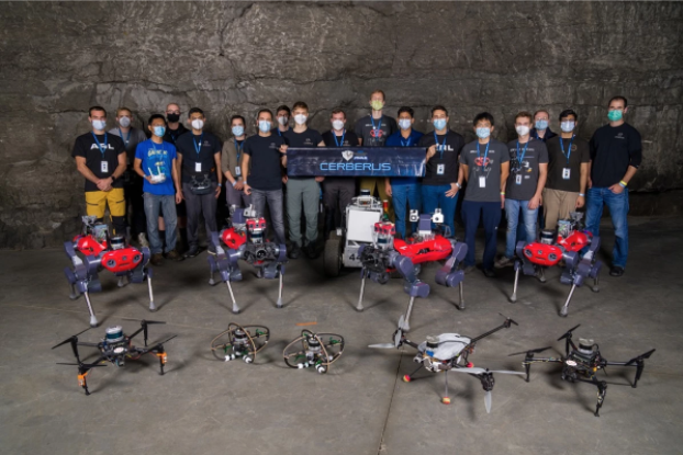
The team participated in the competition with four quadruped robots called ANYmal, five primarily in-house-built drones with variable size and payload capacity, and a rover robot in the form of Super Mega Bot. In the competition finals, the team ended up using four ANYmal robots and the Super Mega Bot for exploration and artifact detection.
Each ANYmal robot was equipped with two CPU-based computers and an NVIDIA Jetson AGX Xavier. The rover robot was equipped with an NVIDIA GTX 1070 GPU.
The CERBERUS team used a modified version of the You Only Look Once (YOLO) model for object detection. The model was trained on 40,000 labeled images using two NVIDIA RTX 3090 GPUs.
The trained model was further optimized using TensorRT before being deployed on Jetson for real-time inference. The Jetson AGX Xavier was able to perform inference at a collective rate of 20 Hz. In the competition finals, the CERBERUS team was the first to detect 23 of the 40 artifacts located in the environment, clinching the number one spot.
The CERBERUS team also used GPUs for the elevation mapping of the terrain and training the locomotion policy controller of the ANYmal quadruple robot. The elevation mapping was done in real-time using Jetson AGX Xavier. The ANYmal robot’s locomotion policy training for the rough terrain was done offline using desktop GPUs.
Team Co-STAR
Led by researchers at NASA’s Jet Propulsion Laboratory (JPL) in Southern California along with other universities and industrial collaborators, team Collaborative SubTerranean Autonomous Robots (Co-STAR) was the winner of the 2020 competition focused on exploring complex underground urban environments.
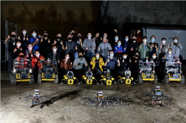
They also successfully participated in the 2021 competition in mixed artificial and natural environments, placing fifth. The Co-STAR team entered the competition with four Spots, four Husky robots, and two drones.
Following an unexpected hardware issue in the final run, the team ended up using one Spot and three Husky robots. Each robot was equipped with a CPU-based computer along with one NVIDIA Jetson AGX Xavier.
For object detection, team Co-STAR used RGB and thermal images. They used the medium variant of the YOLO v5 model to process high-resolution images for real-time inference. The team trained two different models to perform inference on captured RGB and thermal images.
The image-based model was trained using approximately 54,000 labeled frames whereas the thermal image model was trained using about 2,400 labeled images. For training the model on their customized dataset, team Co-STAR used a pretrained YOLO v5 model on the COCO dataset and performed transfer learning using the NVIDIA Transfer Learning Toolkit (known as TAO Toolkit).
The models were trained using two on-premise NVIDIA A100 GPUs and an AWS instance that consisted of eight V100 GPUs. Before deploying the models on Jetson AGX Xavier, the team pruned the models using TensorRT.
Using this setup, team Co-STAR was able to perform inference at 28 Hz with RGB images received from five RealSense cameras and images received from one thermal camera. In the final run, the robots were able to detect all 13 artifacts present in the designated areas. The exploration time was limited due to the delayed deployment caused by unexpected hardware issues at the deployment site.
Equipped with the NVIDIA Jetson platform and NVIDIA GPU hardware, teams competing in the DARPA SubT event were able to effectively train models for real-time inference, addressing the challenge posed by underground environments with accurate object detection.