I am using Dataspell and have a jupyter notebook set up inside dataspell, I’ve done simple imports such as
import TensorFlow as tf
import tensorflow_hub as hub
import tensorflow_text as text
but its has been like 2 hours and it still hasn’t finished loading, I’ve made sure that i already installed the packages using terminal pip install TensorFlow etc
I am trying to build a sorting system to sort parts by taking a picture of the part, identifying the part, and then telling a robot to move the part into the appropriate bucket. 99% of the parts are known and can be trained for. 1% of the parts are not known. I would like the known parts to be put in their buckets, and all of the unknown parts to be rejected into a single bucket called unknown.
I naively thought I would be able to do this with Resnet50 by looking at the weights returned in the prediction array. I thought the predictor would have uncertainty when presented with an unknown part. However, I have discovered that Resnet50 (and perhaps all image classifiers) will force any image to be in one of it’s trained for buckets with a high level of confidence.
Because only 1% of the parts are unknown, I can’t realistically gather enough of them to train for. Furthermore, I don’t know when and where they will show up.
Does anyone know of a technique I could use to sort images of known parts into their buckets, and reject unknown parts?
The greater performance delivered by current-generation NVIDIA GPU-accelerated instances more than outweighs the per-hour pricing differences of prior-generation GPUs.
AI is transforming every industry, enabling powerful new applications and use cases that simply weren’t possible with traditional software. As AI continues to proliferate, and with the size and complexity of AI models on the rise, significant advances in AI compute performance are required to keep up.
That’s where the NVIDIA platform comes in.
With a full-stack approach spanning chips, systems, software, and even the entire data center, NVIDIA delivers both the highest performance and the greatest versatility for all AI workloads, including AI training. NVIDIA demonstrated this in the MLPerf Training v1.1, the latest edition of an industry-standard, peer-reviewed benchmark suite that measures ML training performance across a wide range of networks. Systems powered by the NVIDIA A100 Tensor Core GPU, including the Azure NDm A100 v4 cloud instance, delivered chart-topping results, set new records, and were the only ones to complete all eight MLPerf Training tests.
All major cloud service providers offer NVIDIA GPU-accelerated instances powered by the A100, making the public cloud a great place to tap into the performance and capabilities of the NVIDIA platform. In this post, I show how a strategy of selecting current-generation instances based on the A100 not only delivers the fastest time to train AI models in the cloud but is also the most cost-effective.
NVIDIA A100 turbocharges AI training
The NVIDIA A100 is based on the Ampere architecture, which incorporates a host of innovations that speed up AI training compared to the prior-generation NVIDIA V100, such as third-generation Tensor Cores, a new generation of NVLink, and much greater memory bandwidth. These enhancements deliver a giant performance leap, enabling the reduction in the time to train a wide range of AI networks.
In this post, I use ResNet-50 to represent image classification, BERT Large for natural language processing, and DLRM for recommender systems.
Figure 1. The NVIDIA A100 dramatically reduces the time to train AI models compared to the NVIDIA V100
GPU Server: Dual socket AMD EPYC 7742 @ 2.25GHz w/ 8x NVIDIA A100 SXM4-40GB and Dual socket Intel Xeon E5-2698 v4 @ 2.2GHz w/ 8x NVIDIA V100 SXM2-32GB. Frameworks: TensorFlow for ResNet-50 v1.5, PyTorch for BERT-Large and DLRM; Precision: Mixed+XLA for ResNet-50 v1.5, Mixed for BERT-Large and DLRM. NVIDIA Driver: 465.19.01; Dataset: ImageNet2012 for ResNet-50 v1.5, SQuaD v1.1 for BERT Large Fine Tuning, Criteo Terabyte Dataset for DLRM, Batch sizes for ResNet-50: A100, V100 = 256; Batch sizes for BERT Large: A100 = 32, V100 = 10; Batch sizes for DLRM: A100, V100 = 65536.
Faster training times speed time to insight, maximizing the productivity of an organization’s data science teams and getting the trained network deployed sooner. There’s also another important benefit: lower costs!
Cloud instances are commonly priced per unit of time, with hourly pricing typical for on-demand usage. The cost to train a model is the product of both hourly instance pricing and the time required to train a model.
Although it can be tempting to select the instances with the lowest hourly price, this might not lead to the lowest cost to train. An instance might be slightly cheaper on a per-hour basis but take significantly longer to train a model. The total cost to train is higher than it would be with the higher-priced instance that gets the job done more quickly. In addition, there’s the time lost waiting for the slower instance to complete the training run.
In the performance numbers shown earlier, the NVIDIA A100 can train models much more quickly than NVIDIA V100. That’s almost 3x as fast in the case of BERT Large Fine Tuning. At the same time, A100-based instances from major cloud providers are often only priced at modest premiums to their prior-generation, V100-based counterparts.
In this post, I discuss how using A100-based cloud instances enables you to save time and money while training AI models, compared to V100-based cloud instances.
Translating performance into savings
Given the immense computational demands of AI training, it is common to train models using multiple GPUs working in concert to reduce training times significantly.
The NVIDIA platform has been designed to deliver industry-leading per-accelerator performance and achieve the best performance and highest ROI at scale, thanks to technologies like NVLink and NVSwitch. That’s why, in this post, I estimate the cost savings that instances with eight NVIDIA A100 GPUs can deliver compared to instances with eight NVIDIA V100 GPUs.
For this analysis, I estimate the relative costs to train ResNet-50, fine tune BERT Large, and train DLRM on V100- and A100-based instances from three major cloud service providers: Amazon Web Services, Google Cloud Platform, and Microsoft Azure.
CSP
Instance
GPU Configuration
Amazon Web Services
p4d.24xlarge
8x NVIDIA A100 40GB
p3dn.24xlarge
8x NVIDIA V100 32GB
p3.16xlarge
8x NVIDIA V100 16GB
Google Cloud Platform
a2-highgpu-8g
8x NVIDIA A100 40GB
n1-highmem-96
8x NVIDIA V100 16GB
Microsoft Azure
Standard_ND96asr_v4
8x NVIDIA A100 40GB
ND40rs v2
8x NVIDIA V100 32GB
Table 1. NVIDIA GPU-accelerated instances from AWS, GCP, and Microsoft Azure.
Estimate methodology
To estimate the training performance of the cloud instances, I used measured time to train data on NVIDIA DGX systems with GPU configurations that correspond to those in the instances. As a result of the deep engineering collaboration with these cloud partners, the performance of NVIDIA-powered cloud instances should be similar to the performance achievable on the DGX systems.
Then, with the measured time-to-train data, I used on-demand, per-hour instance pricing to estimate the cost to train ResNet-50, fine tune BERT Large, and train DLRM.
Estimated cost savings
The following charts all tell a similar story: no matter which cloud service provider you choose, selecting instances based on the latest NVIDIA A100 GPUs can translate into significant cost savings when training a range of AI models. This is even though, on a per-hour basis, instances based on the NVIDIA A100 are more expensive than instances using prior-generation V100 GPUs.
Amazon Web Services:
Figure 2. Estimated cost savings for training models using A100 instances on AWS compared to V100 (16GB and 32GB) instances
GPU Server: Dual socket AMD EPYC 7742 @ 2.25GHz w/ 8x NVIDIA A100 SXM4-40GB, Dual socket Intel Xeon E5-2698 v4 @ 2.2GHz w/ 8x NVIDIA V100 SXM2-32GB, and Dual socket Intel Xeon E5-2698 v4 @ 2.2GHz w/ 8x NVIDIA V100 SXM2-16GB. Frameworks: TensorFlow for ResNet-50 v1.5, PyTorch for BERT-Large and DLRM; Precision: Mixed+XLA for ResNet-50 v1.5, Mixed for BERT-Large and DLRM. NVIDIA Driver: 465.19.01; Dataset: Imagenet2012 for ResNet-50 v1.5, SQuaD v1.1 for BERT Large Fine Tuning, Criteo Terabyte Dataset for DLRM, Batch sizes for ResNet-50: A100, V100 = 256; Batch sizes for BERT Large: A100 = 32, V100 = 10; Batch sizes for DLRM: A100, V100 = 65536; Cost estimated using performance data run on the earlier configurations as well as on-demand instance pricing as of 2/8/2022.
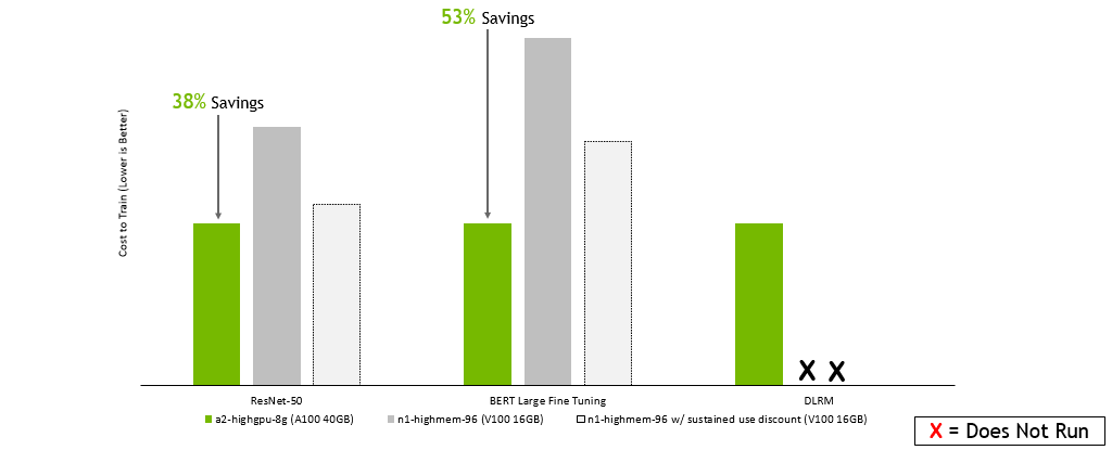
Google Cloud Platform:
Figure 3. Estimated cost savings for training models using A100 instances on GCP compared to V100 (16GB) instances
GPU Server: Dual socket AMD EPYC 7742 @ 2.25GHz w/ 8x NVIDIA A100 SXM4-40GB, Dual socket Intel Xeon E5-2698 v4 @ 2.2GHz w/ 8x NVIDIA V100 SXM2-32GB, and Dual socket Intel Xeon E5-2698 v4 @ 2.2GHz w/ 8x NVIDIA V100 SXM2-16GB. Frameworks: TensorFlow for ResNet-50 v1.5, PyTorch for BERT-Large and DLRM; Precision: Mixed+XLA for ResNet-50 v1.5, Mixed for BERT-Large and DLRM. NVIDIA Driver: 465.19.01; Dataset: ImageNet2012 for ResNet-50 v1.5, SQuaD v1.1 for BERT Large Fine Tuning, Criteo Terabyte Dataset for DLRM, Batch sizes for ResNet-50: A100, V100 = 256; Batch sizes for BERT Large: A100 = 32, V100 = 10; Batch sizes for DLRM: A100, V100 = 65536; Cost estimated using performance data run on the earlier configurations as well as on-demand instance pricing as of 2/8/2022.
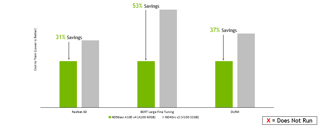
Microsoft Azure:
Figure 4. Estimated cost savings for training models using A100 instances on GCP compared to V100 (32-GB) instances
GPU Server: Dual socket AMD EPYC 7742 @ 2.25GHz w/ 8x NVIDIA A100 SXM4-40GB, Dual socket Intel Xeon E5-2698 v4 @ 2.2GHz w/ 8x NVIDIA V100 SXM2-32GB, and Dual socket Intel Xeon E5-2698 v4 @ 2.2GHz w/ 8x NVIDIA V100 SXM2-16GB. Frameworks: TensorFlow for ResNet-50 v1.5, PyTorch for BERT-Large and DLRM; Precision: Mixed+XLA for ResNet-50 v1.5, Mixed for BERT-Large and DLRM. NVIDIA Driver: 465.19.01; Dataset: ImageNet2012 for ResNet-50 v1.5, SQuaD v1.1 for BERT Large Fine Tuning, Criteo Terabyte Dataset for DLRM, Batch sizes for ResNet-50: A100, V100 = 256; Batch sizes for BERT Large: A100 = 32, V100 = 10; Batch sizes for DLRM: A100, V100 = 65536; Costs estimated using performance data run on the earlier configurations as well as on-demand instance pricing as of 2/8/2022.
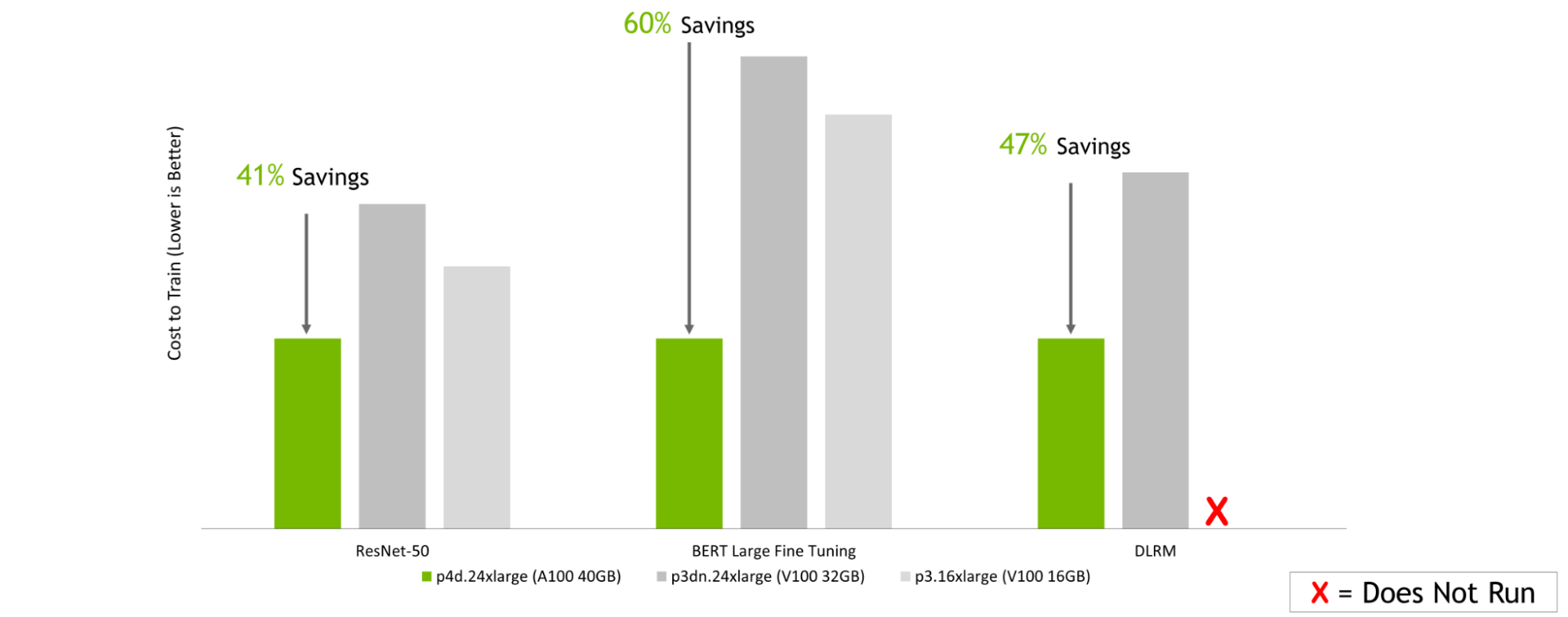
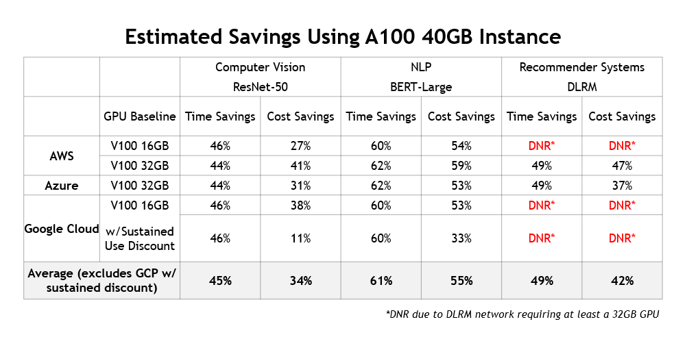
In addition to delivering lower training costs and saving users a significant amount of time, there’s another benefit to using current-generation instances: they enable fundamentally new AI use cases. For example, AI-based recommendation engines are becoming increasingly popular and NVIDIA GPUs are commonly used to train them. Figure 5 summarizes the cost and time savings that A100-instances deliver across different cloud providers:
Figure 5. Time and cost savings of A100-based instances compared to V100 counterparts. Based on on-demand instance pricing as of 2/8/2022.
Higher performance also means higher savings
These results presented here show that the much greater performance delivered by current-generation NVIDIA GPU-accelerated instances more than outweighs the per-hour pricing differences compared to older instances that use prior-generation GPUs.
Instances based on the latest NVIDIA A100 GPUs not only maximize the productivity of your data science teams by minimizing training time, but they’re also the most cost-effective way to train your models in the cloud.
To learn more about the many options for using NVIDIA acceleration in the cloud, see Cloud Computing.
While the current pre-training and fine-tuning action recognition paradigm is straightforward and manifests strong empirical results, it may be overly restrictive for building general-purpose action-recognition models. Compared to a dataset like ImageNet that covers a large range of object recognition classes, action recognition datasets like Kinetics and Something-Something-v2 (SSv2) pertain to limited topics. For example, Kinetics include object-centric actions like “cliff diving” and “ice climbing’ while SSv2 contains object-agnostic activities like ’pretending to put something onto something else.’ As a result, we observed poor performance adapting an action recognition model that has been fine-tuned on one dataset to another disparate dataset.
Differences in objects and video backgrounds among datasets further exacerbate learning a general-purpose action recognition classification model. Despite the fact that video datasets may be increasing in size, prior work suggests significant data augmentation and regularization is necessary to achieve strong performance. This latter finding may indicate the model quickly overfits on the target dataset, and as a result, hinders its capacity to generalize to other action recognition tasks.
In “Co-training Transformer with Videos and Images Improves Action Recognition”, we propose a training strategy, named CoVeR, that leverages both image and video data to jointly learn a single general-purpose action recognition model. Our approach is buttressed by two main findings. First, disparate video datasets cover a diverse set of activities, and training them together in a single model could lead to a model that excels at a wide range of activities. Second, video is a perfect source for learning motion information, while images are great for exploiting structural appearance. Leveraging a diverse distribution of image examples may be beneficial in building robust spatial representations in video models. Concretely, CoVeR first pre-trains the model on an image dataset, and during fine-tuning, it simultaneously trains a single model on multiple video and image datasets to build robust spatial and temporal representations for a general-purpose video understanding model.
Architecture and Training Strategy We applied the CoVeR approach to the recently proposed spatial-temporal video transformer, called TimeSFormer, that contains 24 layers of transformer blocks. Each block contains one temporal attention, one spatial attention, and one multilayer perceptron (MLP) layer. To learn from multiple video and image datasets, we adopt a multi-task learning paradigm and equip the action recognition model with multiple classification heads. We pre-train all non-temporal parameters on the large-scale JFT dataset. During fine-tuning, a batch of videos and images are sampled from multiple video and image datasets. The sampling rate is proportional to the size of the datasets. Each sample within the batch is processed by the TimeSFormer and then distributed to the corresponding classifier to get the predictions.
Compared with the standard training strategy, CoVeR has two advantages. First, as the model is directly trained on multiple datasets, the learned video representations are more general and can be directly evaluated on those datasets without additional fine-tuning. Second, Transformer-based models may easily overfit to a smaller video distribution, thus degrading the generalization of the learned representations. Training on multiple datasets mitigates this challenge by reducing the risk of overfitting.
CoVeR adopts a multi-task learning strategy trained on multiple datasets, each with their own classifier.
Accuracy comparison on Moments-in-Time (MiT) dataset.
Transfer Learning We use transfer learning to further verify the video action recognition performance and compare with co-training on multiple datasets, results are summarized below. Specifically, we train on the source datasets, then fine-tune and evaluate on the target dataset.
We first consider K400 as the target dataset. CoVeR co-trained on SSv2 and MiT improves the top-1 accuracy on K400→K400 (where the model is trained on K400 and then fine-tuned on K400) by 1.3%, SSv2→K400 by 1.7%, and MiT→K400 by 0.4%. Similarly, we observe that by transferring to SSv2, CoVeR achieves 2%, 1.8%, and 1.1% improvement over SSv2→SSv2, K400→SSv2, and MiT→SSv2, respectively. The 1.2% and 2% performance improvement on K400 and SSv2 indicates that CoVeR co-trained on multiple datasets could learn better visual representations than the standard training paradigm, which is useful for downstream tasks.
Comparison of transfer learning the representation learned by CoVeR and standard training paradigm. A→B means the model is trained on dataset A and then fine-tuned on dataset B.
Conclusion In this work, we present CoVeR, a training paradigm that jointly learns action recognition and object recognition tasks in a single model for the purpose of constructing a general-purpose action recognition framework. Our analysis indicates that it may be beneficial to integrate many video datasets into one multi-task learning paradigm. We highlight the importance of continuing to learn on image data during fine-tuning to maintain robust spatial representations. Our empirical findings suggest CoVeR can learn a single general-purpose video understanding model which achieves impressive performance across many action recognition datasets without an additional stage of fine-tuning on each downstream application.
Acknowledgements We would like to thank Christopher Fifty, Wei Han, Andrew M. Dai, Ruoming Pang, and Fei Sha for preparation of the CoVeR paper, Yue Zhao, Hexiang Hu, Zirui Wang, Zitian Chen, Qingqing Huang, Claire Cui and Yonghui Wu for helpful discussions and feedbacks, and others on the Brain Team for support throughout this project.
I can load text data using: tf.keras.utils.text_dataset_from_directory but to use that, each of my “rows” need to be in individual files in their own directory and the label is determined by the directory name.
For the life of me, I can’t figure out how to convert a pandas dataframe into a DataSet.
The dataframe would have some structure like this:
index label unstructured_text 1 1 i like ice cream 2 0 i don't like ice cream 3 1 i'm a little teapot and i'm happy
Is there a practical limit on the size of graph Tensorflow can handle? We are looking at large computation problems that could expand to hundreds of million or billions of nodes in the graph, am wondering if Tensorflow can automatically handle the construction and distributed execution of such large graphs over multiple computers using CPUs? Or we have to manually break the graph into smaller ones before sending to Tensorflow?
Any first-hand experience in handling large graphs are great appreciated, such as the maximum graph size you were able to run in Tensorflow, and any potential pitfalls etc,
GauGAN, an AI demo for photorealistic image generation, allows anyone to create stunning landscapes using generative adversarial networks. Named after post-Impressionist painter Paul Gauguin, it was created by NVIDIA Research and can be experienced free through NVIDIA AI Demos. How to Create With GauGAN The latest version of the demo, GauGAN2, turns any combination of Read article >
Since months I want to implement a VERY basic RNN layer for a project. Its kinda frustrating because 99% of the rest of the project is done. Its only the RNN layer and its a major point of the project.
Using NVIDIA TAO Toolkit and Innotescus’ data curation and analysis platform to improve a popular object detection model’s performance on the person class by over 20%.
AI applications are powered by machine learning models that are trained to predict outcomes accurately based on input data such as images, text, or audio. Training a machine learning model from scratch requires vast amounts of data and a considerable amount of human expertise, often making the process too expensive and time-consuming for most organizations.
Transfer learning is the happy medium between building a custom model from scratch and choosing an off-the-shelf commercial model to integrate into an ML application. With transfer learning, you can select a pretrained model that’s related to your solution and retrain it on data reflecting your specific use case. Transfer learning strikes the right balance between the custom-everything approach (often too expensive) and an off-the-shelf approach (often too rigid) and enables you to build tailored solutions with fewer resources.
The NVIDIA TAO Toolkit enables you to apply transfer learning to pretrained models and create custom, production-ready models without the complexity of AI frameworks. To train these models, high-quality data is a must. While TAO focuses on the model-centric steps of the development process, Innotescus focuses on the data-centric steps.
Innotescus is a web-based platform for annotating, analyzing, and curating robust, unbiased datasets for computer vision–based machine learning. Innotescus helps teams scale operations without sacrificing quality. The platform includes automated and assisted annotation for both images and videos, consensus and review features for QA processes, and interactive analytics for proactive dataset analysis and balancing. Together, Innotescus and the TAO toolkit make it cost effective for organizations to apply transfer learning successfully in custom applications, arriving at high performing solutions in little time.
In this post, we address the challenges of building a robust object detection model by integrating the NVIDIA TAO Toolkit with Innotescus. This solution alleviates several common pain points that businesses encounter when building and deploying commercial solutions.
YOLO object detection model
Your goal in this project is to apply transfer learning to the YOLO object detection model in the TAO toolkit using data curated on Innotescus.
Object detection is the ability to localize and classify objects with a bounding box in an image or video. It is the most widely used application of computer vision technology. Object detection solves many complex, real-world challenges, such as the following:
Context and scene understanding
Automating solutions for smart retail
Autonomous driving
Precision agriculture
Why should you use YOLO for this model? Traditionally, deep learning–based object detectors operate through a two-stage process. In the first stage, the model identifies regions of interest in an image. In the second stage, each of these regions are classified.
Typically, many regions are sent to the classification stage, and because classification is an expensive operation, two-stage object detectors are extremely slow. YOLO stands for “You only look once.” As the name suggests, YOLO can localize and classify simultaneously, leading to highly accurate real-time performance, which is essential for most deployable solutions. In April 2020, the fourth iteration of YOLO was published. It has been tested on a multitude of applications and industries and has proven to be robust.
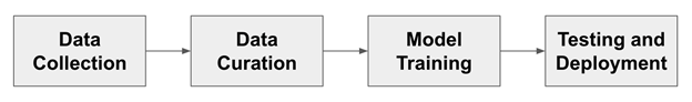
Figure 1 shows the general pipeline for training object detection models. For each step of this more traditional development pipeline, we discuss the typical challenges that people encounter and how the combination of TAO and Innotescus solves these problems.
Figure 1. Typical AI development workflow
Before you begin, install the TAO toolkit and authenticate your instance of the Innotescus API.
Installing TAO Toolkit
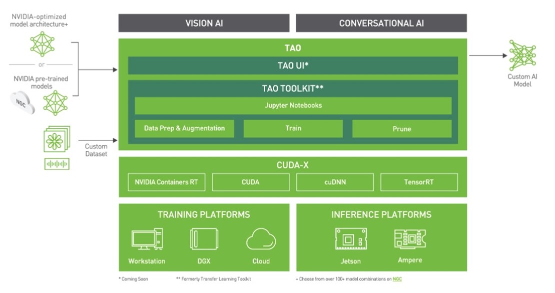
Figure 2. TAO Toolkit stack
The TAO toolkit can be run as a CLI or in a Jupyter notebook. It’s only compatible with Python3 (3.6.9 and 3.7), so first install the prerequisites.
Create an NGC account and generate an API key for authentication.
Log in to the NGC Docker registry by running the command docker login nvcr.io and enter your credentials for authentication.
After the prerequisites are installed, install the TAO toolkit. NVIDIA recommends installing the package in a virtual environment using virtualenvwrapper. To install the TAO launcher Python package, run the following commands:
Check whether you’ve gone through the installation correctly by running tao --help.
Accessing the Innotescus API
Innotescus is accessible as a web-based application, but you’ll also use its API to demonstrate how to accomplish the same tasks programmatically. To begin, install the Innotescus library.
pip install innotescus
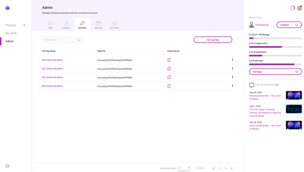
Next, authenticate the API instance using the client_id and client_secret values retrieved from the platform.
Figure 3. Generate and retrieve API keys
from innotescus import client_factory
client = client_factory(client_id=’client_id’, client_secret=’client_secret’)
Now you’re ready to interact with the platform through the API, which you’ll do as you walk through each step of the pipeline that follows.
Data collection
You need data to train the model. Though it’s often overlooked, data collection is arguably the most important step in the development process. While collecting data, you should ask yourself a few questions:
Is the training data adequately representative of each object of interest?
Are you accounting for all the scenarios in which you expect the model to be deployed?
Do you have enough data to train the model?
You can’t always answer these questions completely but having a well-rounded game plan for data collection helps you avoid issues during subsequent steps in the development process. Data collection is a time-consuming and expensive process. Because the models provided by TAO are pretrained, the data requirements for retraining are much smaller, saving organizations significant resources in this phase.
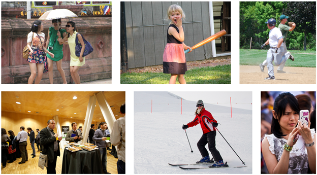
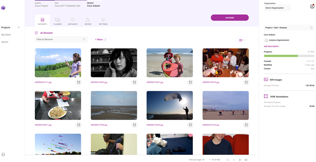
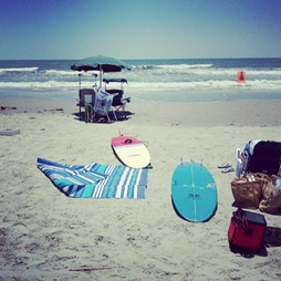
For this experiment, you use images and annotations from the MS COCO Validation 2017 dataset. This dataset has 5,000 images with 80 different classes, but you only use the 2,685 images containing at least one person.
%matplotlib inline
from pycocotools.coco import COCO
import matplotlib.pyplot as plt

dataDir=’Your Data Directory’
dataType=’val2017’
annFile=’{}/annotations/instances_{}.json’.format(dataDir,dataType)

coco=COCO(annFile)

catIds = coco.getCatIds(catNms=[‘person’]) # only using ‘person’ category
imgIds = coco.getImgIds(catIds=catIds)

for num_imgs in len(imgIds):
	img = coco.loadImgs(imgIds[num_imgs])[0]
	I = io.imread(img[‘coco_url’])
Figure 4. Examples of images from the dataset that include one or more ‘person’ objects
With the authenticated instance of the Innotescus client, begin setting up a project and uploading the human-focused dataset.
#create a new project
client.create_project(project_name)
#upload data to the new project
client.upload_data(project_name, dataset_name, file_paths, data_type, storage_type)
data_type: The type of data this dataset holds. Accepted values:
DataType.IMAGE
DataType.VIDEO
storage_type: The source of the data. Accepted values:
StorageType.FILE_SYSTEM
StorageType.URL
This dataset is now accessible through the Innotescus user interface.
Figure 5. Gallery view of the human-centric Coco Validation 2017 dataset from within the Innotescus platform
Data curation
Now that you have your initial dataset, begin curating it to ensure a well-balanced dataset. Studies have repeatedly shown that this phase of the process takes around 80% of the time spent on a machine learning project.
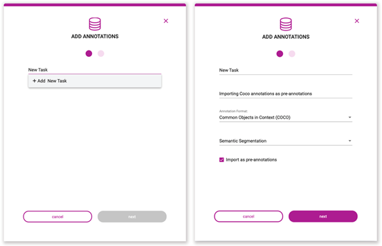
Using TAO and Innotescus, we highlight techniques like pre-annotation and review that save time during this step without sacrificing dataset size or quality.
Pre-annotation
Pre-annotation enables you to use model-generated annotations to remove a significant amount of the time and manual effort necessary to label the subset of 2,685 images accurately. You use YOLOv4—the same model that you’re retraining—to generate pre-annotations for the annotators to refine.
Because pre-annotation saves you so much time on the easier components of the annotation task, you can focus your attention on the harder examples that the model can’t yet handle.
YOLOv4 is included in the TAO toolkit and supports k-means clustering, training, evaluation, inference, pruning, and exporting. To use the model, you must first create a YOLOv4 spec file, which has the following major components:
yolov4_config
training_config
eval_config
nms_config
augmentation_config
dataset_config
The spec file is a protobuf text (prototxt) message, and each of its fields can be either a basic data type or a nested message.
Next, download the model with pretrained weights. The TAO Toolkit Docker container provides access to a repository of pretrained models that serve as a great starting point when training deep neural networks. Because these models are hosted on the NGC catalog, you must first download and install the NGC CLI. For more information, see the NGC documentation.
After you’ve installed the CLI, you can see the list of pretrained computer vision models on the NGC repo, and download pretrained models.
ngc registry model list nvidia/tao/pretrained_*
ngc registry model download-version /path/to/model_on_NGC_repo/ -dest /path/to/model_download_dir/
With the model downloaded and spec file updated, you can now generate pre-annotations by running the inference subtask.
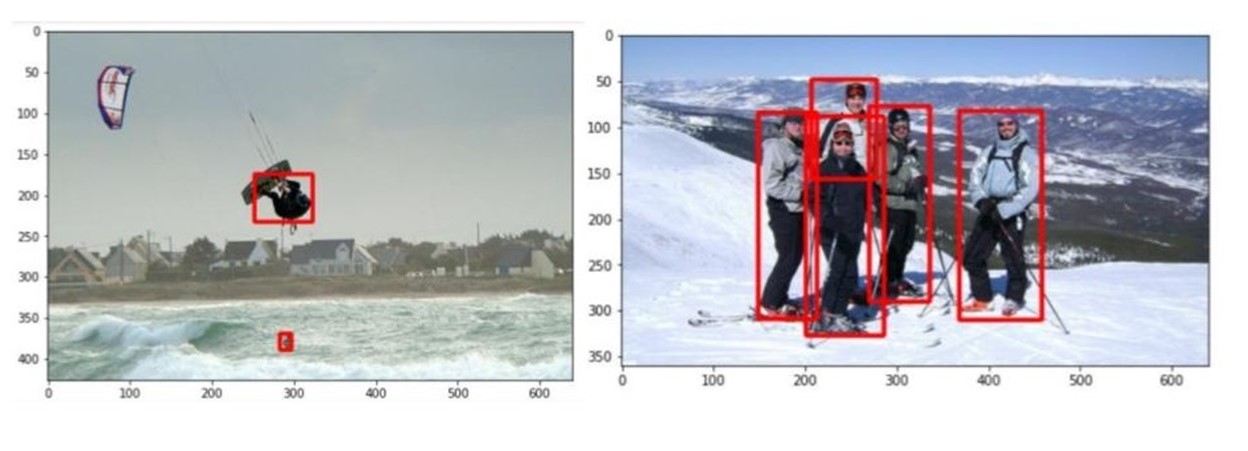
The output of the inference subtask is a series of annotations in the KITTI format, saved in the specified output directory. Figure 6 shows two examples of these annotations:
Figure 6. Example annotations generated by the TAO Toolkit using the pretrained YOLOv4 model
Upload the preannotations into the Innotescus platform manually through the web-based user interface or using the API. Because the KITTI format is one of the many accepted by Innotescus, no preprocessing is needed.
project_name: The name of the project containing the affected dataset and task.
dataset_name: The name of the dataset to which these annotations are to be applied.
task_type: The type of annotation task being created with these annotations. Accepted values from the TaskType class:
CLASSIFICATION
OBJECT_DETECTION
SEGMENTATION
INSTANCE_SEGMENTATION
data_type: The type of data to which the annotations correspond. Accepted values:
DataType.IMAGE
DataType.VIDEO
annotation_format: The format in which these annotations are stored. Accepted values from the AnnotationFormat class:
COCO
KITTI
MASKS_PER_CLASS
PASCAL
CSV
MASKS_SEMANTIC
MASKS_INSTANCE
INNOTESCUS_JSON
YOLO_DARKNET
YOLO_KERAS
file_paths: A list of file paths containing the annotation files to upload.
task_name: The name of the task to which these annotations belong; if the task does not exist, it is created and populated with these annotations.
task_description: A description of the task being created, if the task does not exist yet.
overwrite_existing_annotations: If the task already exists, this flag allows you to overwrite existing annotations.
pre_annotate: Allows you to import annotations as pre-annotations.
With the pre-annotations imported to the platform and a significant amount of the initial annotation work saved, move into Innotescus to further correct, refine, and analyze the data.
Review and correction
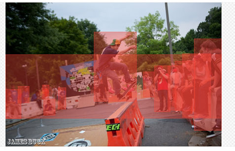
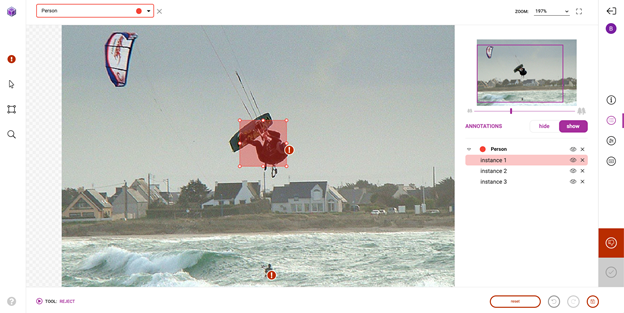
With the pre-annotations successfully imported, head over to the platform to perform review and correction of the pre-annotations. While the pretrained model saves a significant amount of annotation time, it’s still not perfect and needs a bit of human in the loop interaction to ensure high-quality training data. Figure 8 shows an example of a typical correction that you might make.
Figure 8. Error in the pre-annotations generated with the pretrained YOLOv4
Beyond a first pass at fixing and submitting pre-annotations, Innotescus enables a more focused sampling of images and annotations for multistage review. This enables large teams to ensure high quality throughout the dataset systematically and efficiently.
Figure 9. Process on Innotescus
Exploratory data analysis
Exploratory data analysis, or EDA, is the process of investigating and visualizing datasets from multiple statistical angles to get a holistic understanding of the underlying patterns, anomalies, and biases present in the data. It is an effective and necessary step to take before thoughtfully addressing the statistical imbalances your dataset contains.
Innotescus provides precalculated metrics for understanding class, color, spatial, and complexity distributions for both data and annotations, and enables you to add your own layer of information in image and annotation metadata to incorporate application-specific information into the analytics.
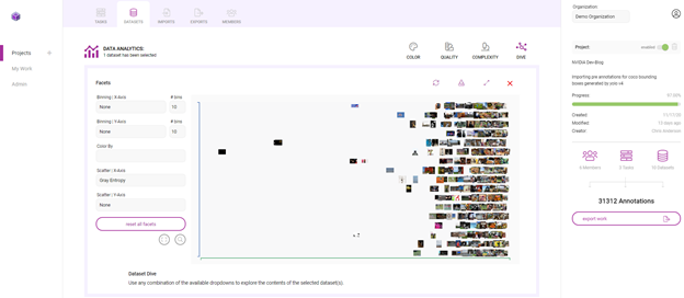
Here’s how you can use the Innotescus’s dive visualization to understand some of the patterns and biases present in the dataset. The following scatter plot shows the distribution of image entropy, which is the average information or degree of randomness in an image, within the dataset along the x-axis. You can see a clear pattern, but you can also spot anomalies like images with low entropy or information content.
Figure 10. Dataset graph on Innotescus
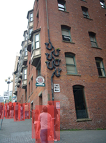
Figure 11. Examples of (left) low- and (right) high-entropy images
Outliers like these raise questions of how to handle anomalies within a dataset. Recognizing anomalies enables you to ask some crucial questions:
Do you expect the model, when deployed, to encounter low-entropy input?
If so, do you need more such examples in the training dataset?
If not, are these examples going to be detrimental for training, and should they be removed from the training dataset?
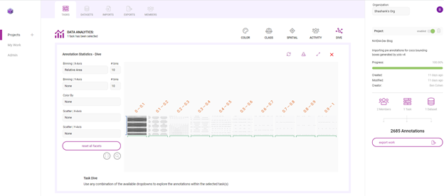
In another example, look at each annotation’s area, relative to the image that it’s in.
Figure 12. Using dive charts to investigate a number of metrics calculated by Innotescus
Figure 13. Variation in relative annotation size within the dataset
In Figure 13, the two images show the variation in annotation sizes within the dataset. While some annotations capture people that take up lots of the image, most show people far away from the camera.
Here, a large percentage of annotations are between 0 and 10% of their respective image sizes. This means that the dataset is biased towards small objects, or people that are far from the camera. Do you then need more examples in the training data that have larger annotations to represent people closer to the camera? Understanding the data distribution in this way helps you to begin thinking about the plan for data augmentation.
With Innotescus, EDA is made intuitive. It provides you with the information that you need to make powerful augmentations to your dataset and eliminate bias early in the development process.
Cluster rebalancing with dataset augmentation
The idea behind augmentation for cluster rebalancing is powerful. This technique showed a 21% boost in performance in the recent datacentric AI competition hosted by Andrew Ng and DeepLearning.AI.
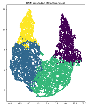
You generate an N-dimensional feature vector for each data point (each bounding box annotation), and cluster all data points in higher dimensional space. When you cluster objects with similar features, you augment the dataset such that each cluster has equal representation.
We chose to use [red channel mean, green channel mean, blue channel mean, gray image std, gray image entropy, relative area] as the N-dimensional feature vector. These metrics were exported from Innotescus, which automatically calculated them. You could also use the embeddings generated by the pretrained model to populate the feature vector, which would arguably be more robust.
You use k-means clustering with k=4 as the clustering algorithm and UMAP for reducing the dimensions to two for visualization. The following code example generates the graph that shows the UMAP plot, color-coded with these four clusters.
import umap
from sklearn.decomposition import PCA
from sklearn.cluster import KMeans

# k-means on the feature vector
kmeans = KMeans(n_clusters=4, random_state=0).fit(featureVector)

# UMAP for dim reduction and visualization
fit = umap.UMAP(n_neighbors=5,
		min_dist=0.2,
		n_components=2,
		metric=’manhattan’)

u = fit.fit_transform(featureVector)

# Plot UMAP components
plt.scatter(u[:,0], u[:,1], c=(kmeans.labels_))
plt.title(‘UMAP embedding of kmeans colours’)
Figure 14. Four clusters, plotted on two dimensions
When you look at the number of objects in each cluster, you can clearly see the imbalance, which informs how you should augment the data for retraining. The four clusters represent 854, 1523, 1481 and 830 images, respectively. Where an image has objects in more than one cluster, group that image in the cluster with most of its objects for augmentation.
clusters = {}

for file, cluster in zip(filename, kmeans.labels_):
	if cluster not in clusters.keys():
		clusters[cluster] = []
		clusters[cluster].append(file)
	else:
		clusters[cluster].append(file)

for numCls in range(0, len(clusters)):
	print(‘Cluster {}: {} objects, {} images’.format(numCls+1, len(clusters[numCls]), len(list(set(clusters[numCls])))))
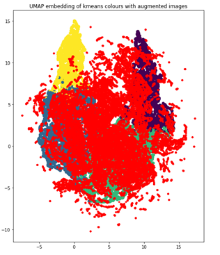
With the clusters well defined, you use the imgaug Python library to introduce augmentation techniques to enhance the training data: translation, image brightness adjustment, and scale augmentation. You augment such that each cluster contains 2,000 images for a total of 8,000. As you augment images, imgaug ensures that the annotation coordinates are altered appropriately as well.
import imgaug as ia
import imgaug.augmenters as iaa

# augment images
seq = iaa.Sequential([
	iaa.Multiply([1.1, 1.5]), # change brightness, doesn’t affect BBs
	iaa.Affine(
		translate_px={“x”:60, “y”:60},
		scale=(0.5, 0.8)
	) # translate by 60px on x/y axes & scale to 50-80%, includes BBs
])

# augment BBs and images
image_aug, bbs_aug = seq(image=I, bounding_boxes=boundingBoxes)
Using the same UMAP visualization technique, with augmented data points now in red, you see that the dataset is now much more balanced, as it more closely resembles a Gaussian distribution.
Figure 15. Rebalanced clusters
Model training
With the well-balanced, high-quality training data, the final step is to train the model.
YOLOv4 retraining on TAO Toolkit
To start retraining the model, first ensure that the spec file contains the classes of interest, as well as the correct directory paths for the pretrained model and training data. Change the training parameters in the training_config section. Reserve 30% of the augmented dataset as a test dataset to compare the performance of the pretrained model and the performance of the retrained model.
tao yolo_v4 train -e /path/to/specFile.txt -r /path/to/result -k $KEY
Results
As you can see, you achieved a 14.93% improvement in the mean average precision, a 21.37% boost from the mAP of the pretrained model:
Model
mAP50
Yolov4 pretrained model
69.86%
Yolov4 retrained model with cluster-rebalanced augmentation
84.79%
Table 1. Model performance before and after applying transfer learning with the curated dataset
Summary
Using NVIDIA TAO Toolkit for pre-annotation and model training and Innotescus for data refinement, analysis, and curation, you improved YOLOv4’s mean average precision on the person class by a substantial amount: over 20%. Not only did you improve the performance on a selected class, you used less time and data than you would have without significant benefits of transfer learning.
Transfer learning is a great way to produce high-performing, application-specific models in settings with constrained resources. Using tools like the TAO toolkit and Innotescus makes it feasible for teams of all sizes and backgrounds.

 The greater performance delivered by current-generation NVIDIA GPU-accelerated instances more than outweighs the per-hour pricing differences of prior-generation GPUs.


 Using NVIDIA TAO Toolkit and Innotescus’ data curation and analysis platform to improve a popular object detection model’s performance on the person class by over 20%.