
Economics, combinatorics, physics, and signal processing conspire to make it difficult to design, build, and operate high-quality, cost-effective wireless networks. The radio transceivers that communicate with our mobile phones, the equipment that supports them (such as power and wired networking), and the physical space they occupy are all expensive, so it’s important to be judicious in choosing sites for new transceivers. Even when the set of available sites is limited, there are exponentially many possible networks that can be built. For example, given only 50 sites, there are 250 (over a million billion) possibilities!
Further complicating things, for every location where service is needed, one must know which transceiver provides the strongest signal and how strong it is. However, the physical characteristics of radio propagation in an environment containing buildings, hills, foliage, and other clutter are incredibly complex, so accurate predictions require sophisticated, computationally-intensive models. Building all possible sites would yield the best coverage and capacity, but even if this were not prohibitively expensive, it would create unacceptable interference among nearby transceivers. Balancing these trade-offs is a core mathematical difficulty.
The goal of wireless network planning is to decide where to place new transceivers to maximize coverage and capacity while minimizing cost and interference. Building an automatic network planning system (a.k.a., auto-planner) that quickly solves national-scale problems at fine-grained resolution without compromising solution quality has been among the most important and difficult open challenges in telecom research for decades.
To address these issues, we are piloting network planning tools built using detailed geometric models derived from high-resolution geographic data, that feed into radio propagation models powered by distributed computing. This system provides fast, high-accuracy predictions of signal strength. Our optimization algorithms then intelligently sift through the exponential space of possible networks to output a small menu of candidate networks that each achieve different desirable trade-offs among cost, coverage, and interference, while ensuring enough capacity to meet demand.
 |
| Example auto-planning project in Charlotte, NC. Blue dots denote selected candidate sites. The heat map indicates signal strength from the propagation engine. The inset emphasizes the non-isotropic path loss in downtown. |
<!–
 |
| Example auto-planning project in Charlotte, NC. Blue dots denote selected candidate sites. The heat map indicates signal strength from the propagation engine. The inset emphasizes the non-isotropic path loss in downtown. |
–>
Radio Propagation
The propagation of radio waves near Earth’s surface is complicated. Like ripples in a pond, they decay with distance traveled, but they can also penetrate, bounce off, or bend around obstacles, further weakening the signal. Computing radio wave attenuation across a real-world landscape (called path loss) is a hybrid process combining traditional physics-based calculations with learned corrections accounting for obstruction, diffraction, reflection, and scattering of the signal by clutter (e.g., trees and buildings).
We have developed a radio propagation modeling engine that leverages the same high-res geodata that powers Google Earth, Maps and Street View to map the 3D distribution of vegetation and buildings. While accounting for signal origin, frequency, broadcast strength, etc., we train signal correction models using extensive real-world measurements, which account for diverse propagation environments — from flat to hilly terrain and from dense urban to sparse rural areas.
While such hybrid approaches are common, using detailed geodata enables accurate path loss predictions below one-meter resolution. Our propagation engine provides fast point-to-point path loss calculations and scales massively via distributed computation. For instance, computing coverage for 25,000 transceivers scattered across the continental United States can be done at 4 meter resolution in only 1.5 hours, using 1000 CPU cores.
 |
 |
| Photorealistic 3D model in Google Earth (top-left) and corresponding clutter height model (top-right). Path profile through buildings and trees from a source to destination in the clutter model (bottom). Gray denotes buildings and green denotes trees. |
Auto-Planning Inputs
Once accurate coverage estimates are available, we can use them to optimize network planning, for example, deciding where to place hundreds of new sites to maximize network quality. The auto-planning solver addresses large-scale combinatorial optimization problems such as these, using a fast, robust, scalable approach.
Formally, an auto-planning input instance contains a set of demand points (usually a square grid) where service is to be provided, a set of candidate transceiver sites, predicted signal strengths from candidate sites to demand points (supplied by the propagation model), and a cost budget. Each demand point includes a demand quantity (e.g., estimated from the population of wireless users), and each site includes a cost and capacity. Signal strengths below some threshold are omitted. Finally, the input may include an overall cost budget.
Data Summarization for Large Instances
Auto-planning inputs can be huge, not just because of the number of candidate sites (tens of thousands), and demand points (billions), but also because it requires signal strengths to all demand points from all nearby candidate sites. Simple downsampling is insufficient because population density may vary widely over a given region. Therefore, we apply methods like priority sampling to shrink the data. This technique produces a low-variance, unbiased estimate of the original data, preserving an accurate view of the network traffic and interference statistics, and shrinking the input data enough that a city-size instance fits into memory on one machine.
Multi-objective Optimization via Local Search
Combinatorial optimization remains a difficult task, so we created a domain-specific local search algorithm to optimize network quality. The local search algorithmic paradigm is widely applied to address computationally-hard optimization problems. Such algorithms move from one solution to another through a search space of candidate solutions by applying small local changes, stopping at a time limit or when the solution is locally optimal. To evaluate the quality of a candidate network, we combine the different objective functions into a single one, as described in the following section.
The number of local steps to reach a local optimum, number of candidate moves we evaluate per step, and time to evaluate each candidate can all be large when dealing with realistic networks. To achieve a high-quality algorithm that finishes within hours (rather than days), we must address each of these components. Fast candidate evaluation benefits greatly from dynamic data structures that maintain the mapping between each demand point and the site in the candidate solution that provides the strongest signal to it. We update this “strongest-signal” map efficiently as the candidate solution evolves during local search. The following observations help limit both the number of steps to convergence and evaluations per step.
 |
| Bipartite graph representing candidate sites (left) and demand points (right). Selected sites are circled in red, and each demand point is assigned to its strongest available connection. The topmost demand point has no service because the only site that can reach it was not selected. The third and fourth demand points from the top may have high interference if the signal strengths attached to their gray edges are only slightly lower than the ones on their red edges. The bottommost site has high congestion because many demand points get their service from that site, possibly exceeding its capacity. |
Selecting two nearby sites is usually not ideal because they interfere. Our algorithm explicitly forbids such pairs of sites, thereby steering the search toward better solutions while greatly reducing the number of moves considered per step. We identify pairs of forbidden sites based on the demand points they cover, as measured by the weighted Jaccard index. This captures their functional proximity much better than simple geographic distance does, especially in urban or hilly areas where radio propagation is highly non-isotropic.
Breaking the local search into epochs also helps. The first epoch mostly adds sites to increase the coverage area while avoiding forbidden pairs. As we approach the cost budget, we begin a second epoch that includes swap moves between forbidden pairs to fine-tune the interference. This restriction limits the number of candidate moves per step, while focusing on those that improve interference with less change to coverage.
 |
| Three candidate local search moves. Red circles indicate selected sites and the orange edge indicates a forbidden pair. |
Outputting a Diverse Set of Good Solutions
As mentioned before, auto-planning must balance three competing objectives: maximizing coverage, while minimizing interference and capacity violations, subject to a cost budget. There is no single correct tradeoff, so our algorithm delegates the final decision to the user by providing a small menu of candidate networks with different emphases. We apply a multiplier to each objective and optimize the sum. Raising the multiplier for a component guides the algorithm to emphasize it. We perform grid search over multipliers and budgets, generating a large number of solutions, filter out any that are worse than another solution along all four components (including cost), and finally select a small subset that represent different tradeoffs.
 |
| Menu of candidate solutions, one per row, displaying metrics. Clicking on a solution turns the selected sites pink and displays a plot of the interference distribution across covered area and demand. Sites not selected are blue. |
Conclusion
We described our efforts to address the most vexing challenges facing telecom network operators. Using combinatorial optimization in concert with geospatial and radio propagation modeling, we built a scalable auto-planner for wireless telecommunication networks. We are actively exploring how to expand these capabilities to best meet the needs of our customers. Stay tuned!
For questions and other inquiries, please reach out to wireless-network-interest@google.com.
Acknowledgements
These technological advances were enabled by the tireless work of our collaborators: Aaron Archer, Serge Barbosa Da Torre, Imad Fattouch, Danny Liberty, Pishoy Maksy, Zifei Tong, and Mat Varghese. Special thanks to Corinna Cortes, Mazin Gilbert, Rob Katcher, Michael Purdy, Bea Sebastian, Dave Vadasz, Josh Williams, and Aaron Yonas, along with Serge and especially Aaron Archer for their assistance with this blog post.


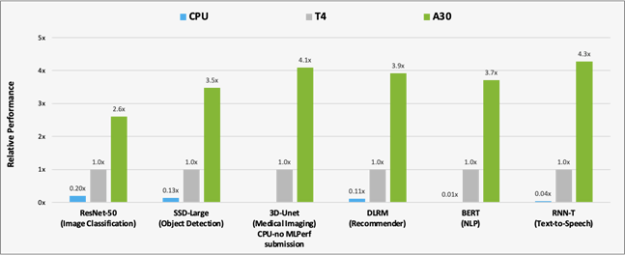
 A30 enables researchers, engineers, and data scientists to deliver real-world results and deploy solutions into production at scale.
 Surface clearing is a widely used accessory operation. This post covers best practices for clears on NVIDIA GPUs.
