Month: May 2022

This post presents an overview of NVIDIA Triton Model Analyzer and how it can be used to find the optimal AI model-serving configuration to satisfy application requirements.

Model deployment is a key phase of the machine learning lifecycle where a trained model is integrated into the existing application ecosystem. This tends to be one of the most cumbersome steps where various application and ecosystem constraints should be satisfied for a target hardware platform, all without compromising the model accuracy. 

NVIDIA Triton Inference Server is an open-source model serving tool that simplifies inference and has several features to maximize hardware utilization and increase inference performance. This includes features like:

• Concurrent model execution, which enables multiple instances of the same model to execute in parallel on the same system.
• Dynamic batching, where client-side requests are grouped together on the server to form a larger batch.

For more information, see Fast and Scalable AI Model Deployment with NVIDIA Triton Inference Server.

There are several key decisions to be made when optimizing model deployment:

• How many model instances should NVIDIA Triton run on the same CPU/GPU concurrently to maximize utilization? 
• How many incoming client requests should be dynamically batched together?
• Which format should the model be served in?
• At what precision should the outputs be computed?

These key decisions lead to a combinatorial explosion, where hundreds of possible configurations are available for each model and hardware choice. Often, this leads to wasted development time or costly subpar serving decisions.

In this post, we explore how the NVIDIA Triton Model Analyzer can automatically sweep through various serving configurations for your target hardware platform and find the best model configurations based on your application’s needs. This can improve developer productivity while increasing the utilization of serving hardware at the same time.

NVIDIA Triton Model Analyzer

NVIDIA Triton Model Analyzer is a versatile CLI tool that helps with a better understanding of the compute and memory requirements of models served through NVIDIA Triton Inference Server. This enables you to characterize the tradeoffs between different configurations and choose the best one for your use case.

NVIDIA Triton Model Analyzer can be used with all the model formats that NVIDIA Triton Inference Server supports: TensorRT, TensorFlow, PyTorch, ONNX, OpenVINO, and others.

You can specify your application constraints (latency, throughput, or memory) to find the serving configurations that satisfy them. For example, a virtual assistant application might have a certain latency budget for the interaction to feel real-time for the end user. An offline processing workflow should be optimized for throughput to reduce the amount of required hardware and to keep the cost as low as possible. The available memory in the model serving hardware may be limited and necessitate the serving configuration to be optimized for memory.

As an example, we take a pretrained model and show how to use NVIDIA Triton Model Analyzer and optimize the serving of this model on a VM instance on Google Cloud Platform. However, the steps shown here can be used on any public cloud or on-premises with any model type that NVIDIA Triton Inference Server supports.

Creating the model

In this post, we use the pretrained BERT Large model from Hugging Face in PyTorch format. NVIDIA Triton Inference Server can serve PyTorch models using its LibTorch backend for TorchScript models or using its Python backend for pure PyTorch models. To get the best performance, we recommend converting PyTorch models to TorchScript format. To this end, use the tracing functionality of PyTorch.

Begin by pulling the PyTorch container from NGC and install the transformers package within the container. If it is your first time using NGC, create an account. We use the 22.04 releases of the relevant tools throughout this post, which were the latest at the time of writing. NVIDIA Triton has a monthly release cadence and ships a new version at the end of every month.

docker pull nvcr.io/nvidia/pytorch:22.04-py3
docker run --rm -it -v $(pwd):/workspace nvcr.io/nvidia/pytorch:22.04-py3 /bin/bash
pip install transformers

When the transformers package is installed, run the following Python code to download the pretrained BERT Large model and trace it into TorchScript format. 

from transformers import BertModel, BertTokenizer
import torch
model_name = "bert-large-uncased"
tokenizer = BertTokenizer.from_pretrained(model_name)
model = BertModel.from_pretrained(model_name, torchscript=True)

max_seq_len = 512
sample = "This is a sample input text"
tokenized = tokenizer(sample, return_tensors="pt", max_length=max_seq_len, padding="max_length", truncation=True)

inputs = (tokenized.data['input_ids'], tokenized.data['attention_mask'], tokenized.data['token_type_ids'])
traced_model = torch.jit.trace(model, inputs)
traced_model.save("model.pt")

Building the model repository

The first step in using NVIDIA Triton Inference Server to serve your models is to create a model repository. In this repository, you include a model configuration file that provides information about the model. At a minimum, a model configuration file must specify the backend, the maximum batch size for the model, and the input/output structure.

For this model, the following code example is the model configuration file. For more information, see Model Configuration.

platform: "pytorch_libtorch"
max_batch_size: 64
input [
  {
    name: "INPUT__0"
    data_type: TYPE_INT64
    dims: [ 512 ]
  },
  {
    name: "INPUT__1"
    data_type: TYPE_INT64
    dims: [ 512 ]
  },
  {
    name: "INPUT__2"
    data_type: TYPE_INT64
    dims: [ 512 ]
  }
]
output [
  {
    name: "OUTPUT__0"
    data_type: TYPE_FP32
    dims: [ -1, 1024 ]
  },
  {
    name: "OUTPUT__1"
    data_type: TYPE_FP32
    dims: [ 1024 ]
  }
]

After naming the model configuration file as config.pbtxt, create a model repository by following the repository layout structure. The folder structure of the model repository should be similar to the following:

.
└── bert-large
    ├── 1
    │   └── model.pt
    └── config.pbtxt

Running NVIDIA Triton Model Analyzer

The recommended way to use Model Analyzer is to build the Docker image for it yourself:

git clone https://github.com/triton-inference-server/model_analyzer.git
cd ./model_analyzer
git checkout r22.04
docker build --pull -t model-analyzer .

Now that you have the Model Analyzer image built, spin up the container:

docker run -it --rm --gpus all 
      -v /var/run/docker.sock:/var/run/docker.sock 
      -v :/models 
      -v :/output 
      -v :/config 
      --net=host model-analyzer

Different hardware configurations might lead to different optimal serving configurations. As such, it is important to run Model Analyzer on the target hardware platform where the models will be eventually served from.

For reproducibility of the results we present in this post, we ran our experiments in the public cloud. Specifically, we used an a2-highgpu-1g instance on Google Cloud Platform with a single NVIDIA A100 GPU.

A100 GPUs support Multi-Instance GPU (MIG), which can maximize the GPU utilization by splitting up a single A100 GPU up to seven partitions with hardware-level isolation that can independently run NVIDIA Triton servers. For the sake of simplicity, we did not use MIG for this post. For more information, see Deploying NVIDIA Triton at Scale with MIG and Kubernetes.

Model Analyzer supports automatic and manual sweeping through different configurations for NVIDIA Triton models. Automatic configuration search is the default behavior and enables dynamic batching for all configurations. In this mode, Model Analyzer sweeps through different batch sizes and the number of instances of a model that can handle incoming requests simultaneously.

The default ranges swept through are up to five instances of a model and up to a batch size of 128. These defaults can be changed.

Now create a configuration file named sweep.yaml to analyze the BERT Large model prepared earlier and perform an automatic sweep through the possible configurations.

model_repository: /models
checkpoint_directory: /output/checkpoints/
output-model-repository-path: /output/bert-large
profile_models:
  bert-large
perf_analyzer_flags:
  input-data: "zero"

Using the preceding configuration, you can get the top line and the bottom line numbers for the model throughput and latency, respectively.

Model Analyzer also writes the collected measurements to checkpoint files when profiling. These are located within the specified checkpoint directory. You can use the profiled checkpoints to create data tables, summaries, and detailed reports of the results.

With the configuration file in place, you are now ready to run Model Analyzer:

model-analyzer profile -f /config/sweep.yaml

As a sample, Table 1 shows a few rows from the results. Each row corresponds to an experiment run on a model configuration under a hypothetical client load.

Model	Batch	Concurrency	Model Config Path	Instance Group	Satisfies Constraints	Throughput (infer/sec)	p99 Latency (ms)
bert-large	1	16	bert-large_config_8	2/GPU	Yes	139	150.9
bert-large	1	32	bert-large_config_8	2/GPU	Yes	128	222.1
bert-large	1	8	bert-large_config_8	2/GPU	Yes	123	79.6
bert-large	1	64	bert-large_config_8	2/GPU	Yes	114	442.6
…	…	…	…	…	…	…	…
bert-large	1	16	bert-large_config_default	1/GPU	Yes	66	219.1

To get a more detailed report of each model configuration tested, use the model-analyzer report command:

model-analyzer report --report-model-configs bert-large_config_default,bert-large_config_1,bert-large_config_2 --export-path /output --config-file /config/sweep.yaml --checkpoint-directory /output/checkpoints/

This generates a report that details the following:

• The hardware the analysis was run on
• A plot of throughput with respect to latency
• A plot of GPU memory with respect to latency
• A report for the chosen configurations in the CLI

This is a great start for any MLOps team to start their analysis before putting a model in production.

Different stakeholders, differing constraints

In a typical production environment, there are multiple teams that should work symbiotically to deploy AI models at a large scale in production. For example, there might be an MLOps team responsible for the model serving pipeline stability and handling the changes in the service-level agreements (SLAs) imposed by the applications. Separately, the infrastructure team is usually responsible for the entire GPU/CPU farm.

Assume that a product team requested that the MLOps team serve BERT Large with 99% of the requests processed within a latency budget of 30 ms. The MLOps team should consider various serving configurations on the available hardware to satisfy that requirement. Using Model Analyzer removes most of the friction in doing so.

The following code example is an example of a configuration file named latency_constraint.yaml, where we added a constraint on the 99th percentile of measured latency values to satisfy the given SLA.

model_repository: /models
checkpoint_directory: /output/checkpoints/
analysis_models: 
  bert-large:
    constraints:
      perf_latency_p99:
        max: 30
perf_analyzer_flags:
  input-data: "zero"

Because you have the checkpoints from the previous sweep, you can reuse them for the SLA analysis. Running the following command gives you the top three configurations satisfying the latency constraint:

model-analyzer analyze -f latency_constraint.yaml

Table 2 shows the measurements taken for the top three configurations and how they compare to the default configuration.

Model Config Name	Max Batch Size	Dynamic Batching	Instance Count	p99 Latency (ms)	Throughput (infer/sec)	Max CPU Memory Usage (MB)	Max GPU Memory Usage (MB)	Average GPU Utilization (%)
bert-large_config_10	1	Enabled	3/GPU	29.278	92.0	0	6026.0	32.1
bert-large_config_5	1	Enabled	2/GPU	24.269	90.0	0	4683.0	23.3
bert-large_config_9	16	Enabled	2/GPU	25.985	90.0	0	4767.0	13.6
bert-large_config_default	64	Disabled	1/GPU	29.14	73.0	0	3268.0	19.2

In large-scale production, the software and the hardware constraints affect the SLA in production.

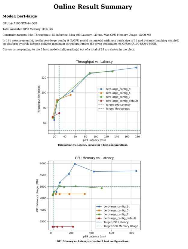
Assume that the constraints of the application have changed. The team would now like to satisfy a p99 latency of 50 ms along with a throughput of 30+ inferences per second for the same model. Also assume that the infrastructure team is able to spare 5,000 MB of GPU memory for its use. Manually finding a serving configuration to satisfy the stakeholders becomes harder and harder as the number of constraints increases. This is where the need for a solution like Model Analyzer becomes more obvious as you can now specify all of our constraints together in a single configuration file.

The following sample configuration file named multiple_constraint.yaml combines throughput, latency, and GPU memory constraints:

model_repository: /models
checkpoint_directory: /output/checkpoints/
analysis_models: 
  bert-large-pytorch:
    constraints:
      perf_throughput:
        min: 50
      perf_latency_p99:
        max: 30
   gpu_used_memory:
        max: 5000
perf_analyzer_flags:
  input-data: "zero"

With this updated constraint in place, run the following command: 

model-analyzer analyze -f multiple_constraint.yaml

Model Analyzer now finds the serving configurations given below as the top three options and shows how they compare to the default configuration.

Model Config Name	Max Batch Size	Dynamic Batching	Instance Count	p99 Latency (ms)	Throughput (infer/sec)	Max CPU Memory Usage (MB)	Max GPU Memory Usage (MB)	Average GPU Utilization (%)
bert-large_config_9	16	Enabled	2/GPU	25.985	90.0	0	4767.0	13.6
bert-large_config_5	1	Enabled	2/GPU	24.269	90.0	0	4683.0	23.3
bert-large_config_7	4	Enabled	2/GPU	25.216	88.0	0	4717.0	38.7
bert-large_config_default	64	Disabled	1/GPU	29.14	73.0	0	3268.0	19.2

NVIDIA Triton Model Analyzer also generates plots and a more detailed report (Figure 2).

Summary

As enterprises find themselves serving more and more models in production, it becomes more and more difficult to make model serving decisions manually or based on heuristics. Doing this manually results in wasted development time or subpar model serving decisions, which necessitates automated tooling.

In this post, we explored how NVIDIA Triton Model Analyzer enables finding model serving configurations satisfying the application SLAs and requirements of various stakeholders. We showed how Model Analyzer can be used to sweep through various configurations, and how it can be used to satisfy specified serving constraints.

Even though we focused on a single model for this post, there are plans to have Model Analyzer perform the same analysis for multiple models at the same time. For example, you could define constraints on different models running on the same GPU and optimize each.

We hope you share our excitement about how much development time Model Analyzer will save and enable your MLOps teams to make well-informed decisions. For more information, see the /triton-inference-server/model_analyzer GitHub repo.

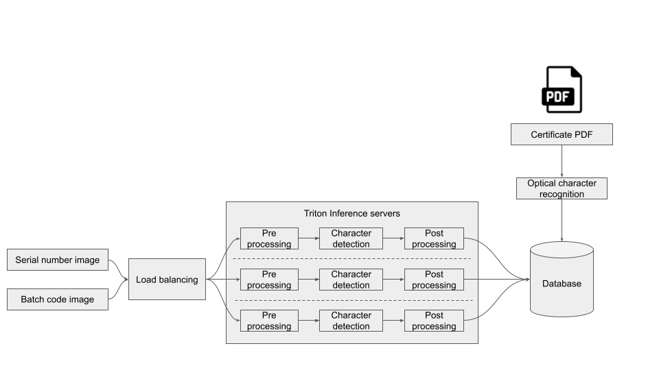
Using an NVIDIA Triton Inference Server, industrial manufacturer Sansera improved quality control and documentation through a custom AI pipeline.

Implementing quality control and assurance methodology in manufacturing processes and quality management systems ensures that end products meet customer requirements and satisfaction. Surface defect detection systems can use image data to perform inspections and classifications for delivering high-quality products. With advancements in AI, real-time defect detection is streamlined and automated using sensors and pretrained AI models for replicable quality control.

Sweden-based company Sansera—a producer of connecting rods for diesel engines—collaborated with AI company Aixia to implement an automated, deep learning defect detection system in their production process using computer vision.

Found in buses, trucks, and ships, every rod in the manufacturing production process must be high quality, consistent, reliable, and documented. It is imperative that the high-resolution, visual inspection system detects and classifies defects in real time.  

To help Sansera reach its manufacturing process quality control goals, Aixia developed and deployed a rod inspection and detection pipeline at Sansera’s production site. At the heart of the pipeline, is an NVIDIA Triton Inference Server deployed on the NVIDIA Jetson edge AI platform and data center servers. It is implemented on an x86 server with NVIDIA A10 GPUs for inference.

Using a quality vision inspection system, robots lift and display connecting rods to a set of AI-enabled cameras. The cameras take multiple photos to capture imprints and serial numbers, which are sent through AI-based computer vision models for inspection in a controlled lighting environment. The evaluations are performed in sequence and the results provide quality control documentation. Several deep learning inferences are performed per camera view.

Each connecting rod is inspected and documented properly before release. The job of this inference workflow is to detect the imprints, inspect their quality, and provide necessary details for the product documentation. The workflow is deployed and optimized on an NVIDIA Triton Inference Server, using different frameworks and consolidates quality use cases in a streamlined fashion. 

Several models, in both pre-and post-processing, are consolidated within one server instance.

Using NVIDIA Triton, Aixia deploys optimized versions of the pretrained models, in the data center using high-performance GPUs, or on the edge close to the data using the Jetson edge AI platform. 

Learn more about how NVIDIA Triton and NVIDIA Jetson can be used to run models at the edge.

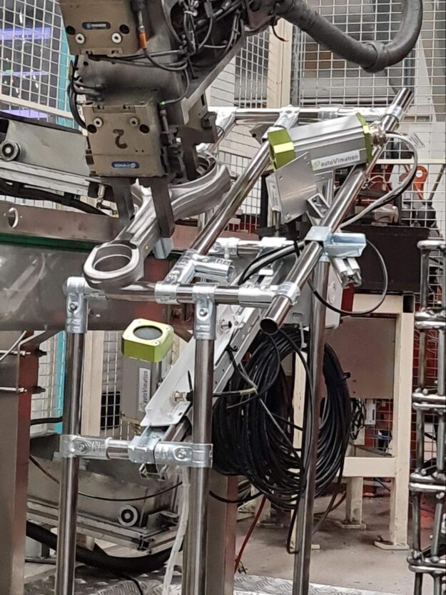
Train highly accurate computer vision models with Lexset synthetic data and the NVIDIA TAO Toolkit.

To develop an accurate computer vision AI application, you need massive amounts of high-quality data. With a traditional dataset, you might spend months collecting images, getting annotations, and cleaning data. When it’s done, you could find edge cases and need more data, starting the cycle all over again.

For years, this cycle has held back AI, especially in computer vision. Lexset builds tools that enable you to generate data to solve this bottleneck. Powerful new workflows with training data can be developed and iterated as part of the AI training cycle.

Lexset’s Seahaven platform generates fully annotated datasets, including photorealistic RGB images, semantic segmentation, and depth maps, in a matter of minutes. Iteration to improve your model’s accuracy is fast and effective. It’s not a months-long process to find data for unusual events or rare conditions anymore. Just quickly adjust your configuration and generate new data to make your model better than ever.

The synthetic data generated from Seahaven can be used to fine-tune and customize pretrained models from the NVIDIA TAO Toolkit. The TAO Toolkit, a low-code AI model development solution, abstracts the complexity of AI frameworks and enables you to create custom, production-ready models for your specific use case with transfer learning.

Reduce time and increase accuracy significantly by using both Seahaven and TAO Toolkit in creating an initial dataset. Most importantly, you can use synthetic data to quickly adapt a model to changing conditions and increased complexity.

Solution overview

For this experiment, you take a simple use case and build a computer vision model capable of finding and differentiating between a common hardware item, such as screws. You start with a simple background and introduce more complexity to show how adaptable synthetic data is to changing conditions.

We created a dataset containing images with annotations of the four screws and used the TAO Toolkit Object Detection model to get started. We used Faster R-CNN, RetinaNet, and YOLOv3.

In this post, I cover the steps required to run this sample dataset, which you can download, through Faster R-CNN. To run RetinaNet or YOLOv3, the steps are the same and are in the provided Jupyter notebook.

I also share how the Lexset synthetic data can be used in concert with model training to quickly address accuracy issues that may arise as use cases become more complex.

To make your own dataset to use with TAO Toolkit, follow the instructions at Using Seahaven and the Seahaven documentation.

To reproduce the results described, follow these main steps:

• Use a pretrained ResNet-18 model and train a ResNet-18 Faster RCNN model on Lexset’s four screws synthetic dataset.
• Use the best trained weights on the synthetic dataset and fine-tune them with 10% of the real-world four-screw dataset.
• Evaluate the best trained and fine-tuned weights on the real screws validation dataset.
• Run inference on the trained model.

Prerequisites

NVIDIA TAO Toolkit requires an NVIDIA GPU (for example, A100) and driver to use their Docker container, so you must have one to proceed.

You also need at least 16 GBs physical RAM, 50 GB of available memory, and an 8-Core. We tested on Python 3.6.9 and used Ubuntu 18.04. TAO Toolkit requires NVIDIA driver 455.xx or later.

• The tao-launcher is strictly a python3-only package, capable of running on Python 3.6.9 or 3.7 or 3.8.
• Install docker-ce by following the official Docker instructions.
• After you have installed docker-ce, follow the post-installation steps to ensure that Docker can be run without sudo.
• Install nvidia-container-toolkit.
• You must have an NGC account and an API key associated with your account. For more information about creating an NGC account and obtaining an API key, see the Installation Prerequisites section.

Download the dataset

Download the dataset from the Google Drive folder (link also provided in the notebook), which contains all the zip files for synthetic and real images of screws.

●	synthetic_dataset_without_complex_phase1.zip
●	synthetic_dataset_with_complex_phase2.zip
●	real_dataset.zip

Extract the dataset inside synthetic_dataset_without_complex_phase1.zip and real_dataset.zip into the /data directory. The dataset directory structure should look like the following:

├── real_test
├── real_train
├── synthetic_test
└── synthetic_train

TAO Toolkit supports datasets in KITTI format, and the provided dataset is already in that format. To verify it further, see KITTI file format.

Environment setup

Create a new virtual environment using virtualenvwrapper. For more information, see Virtual Environments in the Python Guide.

When you have followed the instructions to install virtualenv and virtualenvwrapper, set the Python version:

echo "export VIRTUALENVWRAPPER_PYTHON=/usr/bin/python3" >> ~/.bashrc
source ~/.bashrc
mkvirtualenv launcher -p /usr/bin/python3

Clone the repository:

git clone https://github.com/Lexset/NVIDIA-TAO-Toolkit---Synthetic-Data.git
cd tao-screws

To install the required dependencies for the environment, install the requirements.txt file:

pip3 install -r requirements.txt

Start the Jupyter notebook:

cd faster_rcnn
jupyter notebook --ip 0.0.0.0 --allow-root --port 8888

Setting up TAO Toolkit mounts

The notebook has a script to generate a ~/.tao_mounts.json file.

{
      "Mounts": [
        {
            "source": "ABSOLUTE_PATH_TO_PROJECT_NETWORK_DIRECTORY",
            "destination": "/workspace/tao-experiments"
        },
        {
         "source": "ABSOLUTE_PATH_TO_PROJECT_NETWORK_SPECS_DIRECTORY",
            "destination": "/workspace/tao-experiments/faster_rcnn/specs"
        }
    ],
     "Envs": [
         {
             "variable": "CUDA_VISIBLE_DEVICES",
             "value": "0"
         }
     ],
     "DockerOptions": {
         "shm_size": "16G",
         "ulimits": {
             "memlock": -1,
             "stack": 67108864
         },
         "user": "1001:1001"
     }
 }

The code example generates the global ~/.tao_mounts.json file at the Ubuntu home directory.

Processing the dataset into TFRecords

When the dataset is downloaded and placed in a data directory, the next step is to convert the KITTI files into the TFRecord format used by NVIDIA TAO Toolkit. Generate TFrecords for both the synthetic and real datasets. This code example from the Jupyter notebook generates TFrecords:

#KITTI trainval
!tao faster_rcnn dataset_convert --gpu_index $GPU_INDEX -d $SPECS_DIR/faster_rcnn_tfrecords_kitti_synth_train.txt 
                    -o $DATA_DOWNLOAD_DIR/tfrecords/kitti_synthetic_train/kitti_synthetic_train

!tao faster_rcnn dataset_convert --gpu_index $GPU_INDEX -d $SPECS_DIR/faster_rcnn_tfrecords_kitti_synth_test.txt 
                    -o $DATA_DOWNLOAD_DIR/tfrecords/kitti_synthetic_test/kitti_synthetic_test

The same conversion is applied on the real dataset by the next code example in the notebook.

Download the ResNet-18 convolutional backbone

On the setup of NGC CLI locally, download the convolutional backbone, ResNet-18.

!ngc registry model list nvidia/tao/pretrained_object_detection*

Run a benchmark experiment using synthetic data

The following commands start the training on synthetic data and all the logs are saved on out_resnet18_synth_amp16.log file. To see the logs, open the file or refresh the tab if the file was already opened.

!tao faster_rcnn train --gpu_index $GPU_INDEX -e $SPECS_DIR/default_spec_resnet18_synth_train.txt --use_amp > out_resnet18_synth_amp16.log

Alternatively, you can use the tail command to see the last few lines of the logs.

!tail -f ./out_resnet18_synth_amp16.log

After the training is completed on the synthetic dataset, you can evaluate the synthetically trained model on 10% synthetic validation dataset using the following commands:

!tao faster_rcnn evaluate --gpu_index $GPU_INDEX -e $SPECS_DIR/default_spec_resnet18_synth_train.txt

You see the results like the following.

mAP@0.5 = 0.9986

You also see the individual mAP scores for each class.

Fine-tuning the synthetic-trained model with real data

Now, use the best trained weights from synthetic training and perform the fine-tuning on 10% of the real-world screw dataset. The /train folder inside real_train is already at a 10% split and you can start the fine-tuning using the following commands:

!tao faster_rcnn train --gpu_index $GPU_INDEX -e $SPECS_DIR/default_spec_resnet18_real_train.txt --use_amp > out_resnet18_synth_fine_tune_10_amp16.log

Results: Improvements on 10% of the real data

Per epoch, the mAP score looks like the following data:

mAP@0.5 = 0.9408              
mAP@0.5 = 0.9714              
mAP@0.5 = 0.9732              
mAP@0.5 = 0.9781              
mAP@0.5 = 0.9745              
mAP@0.5 = 0.9780              
mAP@0.5 = 0.9815              
mAP@0.5 = 0.9820              
mAP@0.5 = 0.9803              
mAP@0.5 = 0.9796              
mAP@0.5 = 0.9810              
mAP@0.5 = 0.9817

Fine tuning on just 10% of the real-world screw dataset improves the results quickly and the mAP score above 98%. The features learned from the synthetic dataset helped during the fine-tuning on just 10% of the real-world screw dataset.

Add a complex background in the synthetic screws validation dataset

To further validate the synthetically trained model, we added 300 more images to the complex background dataset. As the initial synthetic dataset was not taken with a complex background, the mean average precision drops significantly.

Just like the real world, as the use case becomes more complex, the accuracy suffers. When validated on images containing more complex or adversarial backgrounds, the mAP score dropped from around 98% to 83.5%. 

Retrain the synthetic dataset with complex backgrounds

This is where synthetic data really shines. To mitigate the loss in mAP when validated on complex images, I generated additional images with more complex backgrounds to add to the training data. I just adjusted the backgrounds so that the new training data set was ready in a manner of seconds. After being introduced, the new dataset boosted performance by an incredible 10-12% with no additional changes.

The dataset with the complex backgrounds is inside the zip file synthetic_dataset_with_complex.zip mentioned earlier. Extract this file and replace the folders inside the /data directory with the same names to have an updated synthetic dataset with a complex background.

Average Mean Precision:
mAP= 94.97%

Increase in mAP score: 11.47%

Specifically, the accuracy of the system with complex backgrounds rose as much as 11.47%, to 94.97%, after just a few minutes of work.

Conclusion

The results showed just how effective and quick it is to iterate with synthetic data and the TAO Toolkit. Using Lexset’s Seahaven, you can generate new data in a matter of minutes and use it to resolve the accuracy issues encountered with introduced complex backgrounds.

The importance of the synthetic dataset is now clear, as the performance of the fine-tuned model on the 90% validation dataset for real-world screw data is extremely good. Use a synthetic dataset for initial feature learning when you have less actual or real-world data. Synthetic datasets can save significant time and cost while producing superior results.

I believe this is the future of computer vision development, where data production occurs in tandem with model iteration. This will give greater controls to the user and enabling you to build the best systems the world has ever seen.

Get started by downloading the Jupyter notebook and sample dataset.

To create your own data, sign up for an account with Lexset.

Demonstrate your computer vision expertise by mastering cloud services, AutoML, and Transformer architectures.

Computer vision is a rapidly growing field in research and applications. Advances in computer vision research are now more directly and immediately applicable to the commercial world.

AI developers are implementing computer vision solutions that identify and classify objects and even react to them in real time. Image classification, face detection, pose estimation, and optical flow are some of the typical tasks. Computer vision engineers are a subset of deep learning (DL) or machine learning (ML) engineers that program computer vision algorithms to accomplish these tasks.

The structure of DL algorithms lend themselves well to solving computer vision problems. The architectural characteristics of convolutional neural networks (CNNs) enable the detection and extraction of spatial patterns and features present in visual data.

The field of computer vision is rapidly transforming industries like automotive, healthcare, and robotics, and it can be difficult to stay up-to-date on the latest discoveries, trends, and advancements. This post highlights the core technologies that are influencing and will continue to shape the future of computer vision development in 2022 and beyond:

• Cloud computing services that help scale DL solutions.
• Automated ML (AutoML) solutions that reduce the repetitive work required in a standard ML pipeline.
• Transformer architectures developed by researchers that optimize computer vision tasks.
• Mobile devices incorporating computer vision technology.

Cloud computing

Cloud computing provides data storage, application servers, networks, and other computer system infrastructure to individuals or businesses over the internet. Cloud computing solutions offer quick, cost-effective, and scalable on-demand resources.

Storage and high processing power are required for most ML solutions. The early-phase development of dataset management (aggregation, cleaning, and wrangling) often requires cloud computing resources for storage or access to solution applications like BigQuery, Hadoop, or BigTable.

Recently, there has been a notable increase in devices and systems enabled with computer vision capabilities, such as pose estimation for gait analysis, face recognition for smartphones, and lane detection in autonomous vehicles.

The demand for cloud storage is growing rapidly, and it is projected that this industry will be valued at $390.33B—five times the market’s current value in 2021. The increased market size will lead to an increase in the use of inbound data to train ML models. This correlates directly to larger data storage capacity requirements and increasingly more powerful compute resources.

GPU availability has accelerated computer vision solutions. However, GPUs alone aren’t always enough to provide the scalability and uptime required by these applications, especially when servicing thousands or even millions of consumers. Cloud computing provides the needed resources to startup and supplement existing on-premises infrastructure gaps.

Cloud computing platforms, including Amazon Web Services (AWS), Google Cloud Platform (GCP), and Microsoft Azure, provide end-to-end solutions to core components of the ML and data science project pipeline, including data aggregation, model implementation, deployment, and monitoring. For computer vision developers designing vision systems, it’s important to be aware of these major cloud service providers their strengths, and how they can be configured to meet specific and complex pipeline needs.

Computer vision at scale requires cloud service integration

The following are examples of NVIDIA services that support typical computer vision systems.

The NGC Catalog of pretrained DL models reduces the complexity of model training and implementation.

DL scripts provide ready-made customizable pipelines. The robust model deployment solution automates delivery to end users.

NVIDIA Triton Inference Server enables the deployment of models from frameworks such as TensorFlow and PyTorch on any GPU– or CPU-based infrastructure. Triton Inference Server provides scalability of models across various platforms, including cloud, edge, and embedded devices.

The NVIDIA partnership with cloud service providers such as AWS enables the deployment of computer vision-based assets, so computer vision engineers can focus more on model performance and optimization.

Businesses reduce costs and optimize strategies wherever feasible. Cloud computing and cloud service providers accomplish both by providing billed solutions based on usage and scaling based on demand.

AutoML

ML algorithms and model development involve a number of tasks that can benefit from automation like, feature engineering and model selection.

Feature engineering involves the detection and selection of relevant characteristics, properties, and attributes from datasets.

Model selection involves evaluating the performance of a group of ML classifiers, algorithms, or solutions to a given problem.

Both feature engineering and model selection activities require considerable time for ML engineers and data scientists to complete. Software developers frequently revisit these phases of the workflow to enhance model performance or accuracy.

There are several large ongoing projects to simplify the intricacies of an ML project pipeline. AutoML focuses on automating and augmentation workflows and their procedures to make ML easy accessible, and less manually intensive for non-ML experts.

Looking at the market value, projections expect the AutoML market to reach $14 billion by 2030. This would mean an increase ~42x higher than its current value.

This particular marriage of ML and automation is gaining traction, but there are limitations.

AutoML in practice

AutoML saves data scientists and computer engineers time. AutoML capabilities enable computer vision developers to dedicate more effort to other phases of the computer vision development pipeline that best use their skillset like model training, evaluation, and deployment. AutoML helps accelerate data aggregation, preparation, and hyperparameter optimization, but these parts of the workflow still require human input.

Data preparation and aggregation are needed to build the right model, but they are repetitive, time-consuming tasks that depend on locating appropriate data quality sources.

Likewise, hyperparameter tuning can take a lot of time to iterate to get the right algorithm performance. It involves a trial-and-error process with educated guesses. The amount of repeated work that goes into finding the appropriate hyperparameters can be tedious but critical for enabling the model’s training to achieve the desired accuracy.

For those interested in exploring GPU-powered AutoML, the widely used Tree-based Pipeline Optimization Tool (TPOT) is an automated ML library aimed at optimizing ML processes and pipelines through the utilization of genetic programming. RAPIDS cuML provides TPOT functionalities accelerated with GPU compute resources. For more information, see Faster AutoML with TPOT and RAPIDS.

Machine learning libraries and frameworks

ML libraries and frameworks are essential elements in any computer vision developer’s toolkit. Major DL libraries such as TensorFlow, PyTorch, Keras, and MXNet received continuous updates and fixes in 2021, and will likely continue to do so in the future.

More recently, there have been exciting advances going on in mobile-focused DL libraries and packages that optimize commonly used DL libraries.

MediaPipe extended its pose estimation capabilities in 2021 to provide 3D pose estimation through the BlazePose model, and this solution is available in the browser and on mobile environments. In 2022, expect to see more pose estimation applications in use cases involving dynamic movement and those that require robust solutions, such as motion analysis in dance and virtual character motion simulation.

PyTorch Lightning is becoming increasingly popular among researchers and professional ML practitioners due to its simplicity, abstraction of complex neural network implementation details, and augmentation of hardware considerations.

State-of-the-art deep learning

DL methods have long been used to tackle computer vision challenges. Neural network architectures for face detection, lane detection, and pose estimation all use deep consecutive layers of CNNs. A new architecture for computer vision algorithms is emerging: transformers.

The Transformer is a DL architecture introduced in Attention Is All You Need. The paper methodology creates a computational representation of data by using the attention mechanism to derive the significance of one part of the input data relative to other segments of the input data.

The Transformer does not use the conventions of CNNs, but research has shown the applications of transformer models in vision-related tasks. Transformers have made a considerable impact within the NLP domain. For more information, see Generative Pre-trained Transformer (GPT) and Bidirectional Encoder Representation From Transformer (BERT).

Explore a transformer model through the NGC Catalog that includes details of the architecture and utilization of an actual transformer model in PyTorch.

For more information about applying the Transformer network architecture to computer vision, see the Transformers in Vision: A Survey paper.

Mobile devices

Edge devices are becoming increasingly powerful. On-device inference capabilities are a must-have feature for mobile applications used by customers who expect quick service delivery and AI features.

The incorporation of computer vision-enabling functionalities within mobile devices, like image and pattern recognition, reduces the latency for obtaining model inference results and provides benefits such as the following:

• Reduced waiting time for obtaining inference results due to on-device computing.
• Enhanced privacy and security due to the limited transfer of data between and to cloud servers.
• Reduced cost of removing dependencies on cloud GPU and the CPU server for inference.

Many businesses are exploring mobile offerings, which includes exploring how existing AI functionality can be replicated on mobile devices. Here are several platforms, tools, and frameworks to implement mobile-first AI solutions:

• TensorFlow Lite
• CoreML
• Apple Vision Framework
• TensorFlow-React
• CreateML
• MediaPipe
• MLKit

Summary

Computer vision technology continues to increase as AI becomes more integrated in our daily lives. Computer vision is also becoming more and more common in the latest news headlines. As this technology scales, the demand for specialists with knowledge in computer vision systems will also rise due to trends in cloud computing service, Auto ML pipelines, transformers, mobile-focused DL libraries, and computer vision mobile applications.

In 2022, increased development in augmented and VR applications will enable computer vision developers to extend their skills into new domains, like developing intuitive and efficient methods of replicating and interacting with real objects in a 3D space. Looking ahead, computer vision applications will continue to change and influence the future.

submitted by /u/TwinnieH
[visit reddit] [comments]

Electric utilities are taking a course in machine learning to create smarter grids for tough challenges ahead. The winter 2021 megastorm in Texas left millions without power. Grid failures the past two summers sparked devastating wildfires amid California’s record drought. “Extreme weather events of 2021 highlighted the risks climate change is introducing, and the importance Read article >

The post Energy Grids Plug into AI for a Brighter, Cleaner Future appeared first on NVIDIA Blog.

submitted by /u/Intelligent-Aioli-43
[visit reddit] [comments]

​Join us on June 16 to take a deep dive into AI at the edge and learn how you can build an edge computing solution that delivers real-time results.

Advances in extended reality have already changed the way we work, live and play, and it’s just getting started. Extended reality, or XR, is an umbrella category that covers a spectrum of newer, immersive technologies, including virtual reality, augmented reality and mixed reality. From gaming to virtual production to product design, XR has enabled people Read article >

The post What is Extended Reality? appeared first on NVIDIA Blog.