On October 18, learn how to unlock one-third of AI compute on the NVIDIA Jetson AGX Orin by leveraging Deep Learning Accelerator for your embedded AI…
On October 18, learn how to unlock one-third of AI compute on the NVIDIA Jetson AGX Orin by leveraging Deep Learning Accelerator for your embedded AI applications.
This self-paced, free tutorial provides a basic understanding of the NVIDIA Isaac Sim interface and the documentation needed to begin robot simulation projects.
This self-paced, free tutorial provides a basic understanding of the NVIDIA Isaac Sim interface and the documentation needed to begin robot simulation projects.
Back in 2018, BERT got people talking about how machine learning models were learning to read and speak. Today, large language models, or LLMs, are growing up fast, showing dexterity in all sorts of applications. They’re, for one, speeding drug discovery, thanks to research from the Rostlab at Technical University of Munich, as well as Read article >
Posted by Zalán Borsos, Research Software Engineer, and Neil Zeghidour, Research Scientist, Google Research
Generating realistic audio requires modeling information represented at different scales. For example, just as music builds complex musical phrases from individual notes, speech combines temporally local structures, such as phonemes or syllables, into words and sentences. Creating well-structured and coherent audio sequences at all these scales is a challenge that has been addressed by coupling audio with transcriptions that can guide the generative process, be it text transcripts for speech synthesis or MIDI representations for piano. However, this approach breaks when trying to model untranscribed aspects of audio, such as speaker characteristics necessary to help people with speech impairments recover their voice, or stylistic components of a piano performance.
In “AudioLM: a Language Modeling Approach to Audio Generation”, we propose a new framework for audio generation that learns to generate realistic speech and piano music by listening to audio only. Audio generated by AudioLM demonstrates long-term consistency (e.g., syntax in speech, melody in music) and high fidelity, outperforming previous systems and pushing the frontiers of audio generation with applications in speech synthesis or computer-assisted music. Following our AI Principles, we’ve also developed a model to identify synthetic audio generated by AudioLM.
From Text to Audio Language Models In recent years, language models trained on very large text corpora have demonstrated their exceptional generative abilities, from open-ended dialogue to machine translation or even common-sense reasoning. They have further shown their capacity to model other signals than texts, such as natural images. The key intuition behind AudioLM is to leverage such advances in language modeling to generate audio without being trained on annotated data.
However, some challenges need to be addressed when moving from text language models to audio language models. First, one must cope with the fact that the data rate for audio is significantly higher, thus leading to much longer sequences — while a written sentence can be represented by a few dozen characters, its audio waveform typically contains hundreds of thousands of values. Second, there is a one-to-many relationship between text and audio. This means that the same sentence can be rendered by different speakers with different speaking styles, emotional content and recording conditions.
To overcome both challenges, AudioLM leverages two kinds of audio tokens. First, semantic tokens are extracted from w2v-BERT, a self-supervised audio model. These tokens capture both local dependencies (e.g., phonetics in speech, local melody in piano music) and global long-term structure (e.g., language syntax and semantic content in speech, harmony and rhythm in piano music), while heavily downsampling the audio signal to allow for modeling long sequences.
However, audio reconstructed from these tokens demonstrates poor fidelity. To overcome this limitation, in addition to semantic tokens, we rely on acoustic tokens produced by a SoundStream neural codec, which capture the details of the audio waveform (such as speaker characteristics or recording conditions) and allow for high-quality synthesis. Training a system to generate both semantic and acoustic tokens leads simultaneously to high audio quality and long-term consistency.
Training an Audio-Only Language Model AudioLM is a pure audio model that is trained without any text or symbolic representation of music. AudioLM models an audio sequence hierarchically, from semantic tokens up to fine acoustic tokens, by chaining several Transformer models, one for each stage. Each stage is trained for the next token prediction based on past tokens, as one would train a text language model. The first stage performs this task on semantic tokens to model the high-level structure of the audio sequence.
In the second stage, we concatenate the entire semantic token sequence, along with the past coarse acoustic tokens, and feed both as conditioning to the coarse acoustic model, which then predicts the future tokens. This step models acoustic properties such as speaker characteristics in speech or timbre in music.
In the third stage, we process the coarse acoustic tokens with the fine acoustic model, which adds even more detail to the final audio. Finally, we feed acoustic tokens to the SoundStream decoder to reconstruct a waveform.
After training, one can condition AudioLM on a few seconds of audio, which enables it to generate consistent continuation. In order to showcase the general applicability of the AudioLM framework, we consider two tasks from different audio domains:
Speech continuation, where the model is expected to retain the speaker characteristics, prosody and recording conditions of the prompt while producing new content that is syntactically correct and semantically consistent.
Piano continuation, where the model is expected to generate piano music that is coherent with the prompt in terms of melody, harmony and rhythm.
In the video below, you can listen to examples where the model is asked to continue either speech or music and generate new content that was not seen during training. As you listen, note that everything you hear after the gray vertical line was generated by AudioLM and that the model has never seen any text or musical transcription, but rather just learned from raw audio. We release more samples on this webpage.
To validate our results, we asked human raters to listen to short audio clips and decide whether it is an original recording of human speech or a synthetic continuation generated by AudioLM. Based on the ratings collected, we observed a 51.2% success rate, which is not statistically significantly different from the 50% success rate achieved when assigning labels at random. This means that speech generated by AudioLM is hard to distinguish from real speech for the average listener.
Our work on AudioLM is for research purposes and we have no plans to release it more broadly at this time. In alignment with our AI Principles, we sought to understand and mitigate the possibility that people could misinterpret the short speech samples synthesized by AudioLM as real speech. For this purpose, we trained a classifier that can detect synthetic speech generated by AudioLM with very high accuracy (98.6%). This shows that despite being (almost) indistinguishable to some listeners, continuations generated by AudioLM are very easy to detect with a simple audio classifier. This is a crucial first step to help protect against the potential misuse of AudioLM, with future efforts potentially exploring technologies such as audio “watermarking”.
Conclusion We introduce AudioLM, a language modeling approach to audio generation that provides both long-term coherence and high audio quality. Experiments on speech generation show not only that AudioLM can generate syntactically and semantically coherent speech without any text, but also that continuations produced by the model are almost indistinguishable from real speech by humans. Moreover, AudioLM goes well beyond speech and can model arbitrary audio signals such as piano music. This encourages the future extensions to other types of audio (e.g., multilingual speech, polyphonic music, and audio events) as well as integrating AudioLM into an encoder-decoder framework for conditioned tasks such as text-to-speech or speech-to-speech translation.
Acknowledgments The work described here was authored by Zalán Borsos, Raphaël Marinier, Damien Vincent, Eugene Kharitonov, Olivier Pietquin, Matt Sharifi, Olivier Teboul, David Grangier, Marco Tagliasacchi and Neil Zeghidour. We are grateful for all discussions and feedback on this work that we received from our colleagues at Google.
Cooler weather, the changing colors of the leaves, the needless addition of pumpkin spice to just about everything, and discount Halloween candy are just some things to look forward to in the fall. GeForce NOW members can add one more thing to the list — 25 games joining the cloud gaming library in October, including Read article >
Thanks to earbuds, people can take calls anywhere, while doing anything. The problem: those on the other end of the call can hear all the background noise, too, whether it’s the roommate’s vacuum cleaner or neighboring conversations at a café. Now, work by a trio of graduate students at the University of Washington, who spent Read article >
When not engrossed in his studies toward a Ph.D. in statistics, conducting data-driven research on AI and robotics, or enjoying his favorite hobby of sailing, Yizhou Zhao is winning contests for developers who use NVIDIA Omniverse — a platform for connecting and building custom 3D pipelines and metaverse applications.
Machine learning (ML) is increasingly used across industries. Fraud detection, demand sensing, and credit underwriting are a few examples of specific use…
Machine learning (ML) is increasingly used across industries. Fraud detection, demand sensing, and credit underwriting are a few examples of specific use cases.
These machine learning models make decisions that affect everyday lives. Therefore, it’s imperative that model predictions are fair, unbiased, and nondiscriminatory. Accurate predictions become vital in high-risk applications where transparency and trust are crucial.
One way to ensure fairness in AI is to analyze the predictions obtained from a machine learning model. This exposes disparities and provides the opportunity to take corrective actions to diagnose and rectify the underlying cause.
Explainable AI (XAI) is a field of Responsible AI dedicated to studying techniques that explain how a machine learning model makes predictions. These explanations are human-understandable, enabling all stakeholders to make sense of the model’s output and make the necessary decisions. SHAP is one such technique used widely in industry to evaluate and explain a model’s prediction.
This post explains how you can train an XGBoost model, implement the SHAP technique in Python using a CPU and GPU, and finally compare results between the two. By the end of the post, you should be able to answer the following questions:
Why is it crucial to explain machine learning models, especially in high-stakes decisions?
How do we differentiate between Interpretable and Explainable techniques?
What is the SHAP technique, and how is it used to explain a model’s predictions?
What is the advantage of GPU-accelerated SHAP?
Explainability versus interpretability
In the context of artificial intelligence and machine learning, it is helpful to distinguish explainability from interpretability. The terms have distinct meanings but are often used interchangeably.
Explainability is a low-level, detailed mental representation that seeks to describe some complex processes. An explanation describes how some model mechanism or output came to be.
Interpretability
Interpretability is a high-level, meaningful mental representation that contextualizes a stimulus and leverages human background knowledge. An interpretable model should provide users with a description of what a data point or model output means in context.
The approaches to explaining model predictions can be broadly divided into model-specific and post-hoc techniques.
Model-specific
Algorithms like generalized linear models, decision trees, and generalized additive models are designed to be interpretable. These are called glassbox models because it is possible to trace and reason how a prediction was made. The techniques used to explain such models are model-specific because each method is based on some specific model’s internals. For instance, the interpretation of weights in linear models counts toward model-specific explanations.
Post-hoc
Post-hoc explainability techniques, as the name suggests, are applied after a model has been trained. Some well-known post-hoc techniques include SHAP, LIME, and Partial Dependence Plots. These are model agnostic. They work by treating the model as a BlackBox and assume they only have access to the model’s inputs and outputs. This makes them beneficial for complex algorithms, like boosted trees and deep neural nets, which are not explainable through model-specific techniques.
This post focuses on SHAP, a post-hoc technique for explaining model predictions.
Using the SHAP technique to explain models
SHAP is an acronym for SHapley Additive Explanations. It is one of the most commonly used post-hoc explainability techniques. SHAP leverages the concept of cooperative game theoryto break down a prediction to measure the impact of each feature on the prediction.
Shapley values are defined as the average marginal contribution of a feature value across all possible feature coalitions. A technique with origins in economics and game theory, Shapley values assign fair payouts to players in a coalition depending upon their contribution to the total gain. Translating this into a machine learning scenario means assigning importance to features in a model depending on their contribution to the model’s prediction.
SHAP unifies several approaches to generate accurate local feature importance values using Shapley values which can then be aggregated to obtain global explanations. SHAP values interpret the impact on the model’s prediction of a given feature having a specific value, compared to the prediction we’d make if that feature took some baseline value. A baseline value is a value that the model would predict if it had no information about any feature values.
SHAP is one of the most widely used post-hoc explainability technique for calculating feature attributions. It is model agnostic, can be used both as a local and global feature attribution technique and has credible theoretical support from economics. Additionally, a variant of SHAP for tree based models reduces the computation time considerably, thereby helping users to gain insights from models quickly.
The following section provides an example of how to use the SHAP technique.
Step 1: Training an XGBoost model and calculating SHAP values
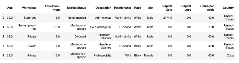
Train an XGBoost model on the given dataset to predict whether a person earns more than $50K a year. Such data could be helpful in various use cases like target marketing.
Compute the SHAP values to explain the individual feature contributions.
Visualize and interpret the SHAP values.
Installation
SHAP can be installed using its stand-alone Python package called shap available on GitHub:
pip install shap

or
conda install -c conda-forge shap
SHAP is also inherently supported by popular algorithms like LightGBM, and XGBoost, and several R packages.
Setting up the environment
Start by setting up the environment and importing the necessary libraries:
import numpy as np
import pandas as pd

# Visualization Libraries
import matplotlib.pyplot as plt
%matplotlib inline

## Machine learning packages
from sklearn.model_selection import train_test_split
import xgboost as xgb

## Model Interpretation package
import shap
shap.initjs()

# Ensuring Reproducibility
SEED = 12345

# Ignoring the warnings
import warnings
warnings.filterwarnings(action = "ignore")
Dataset
This dataset comes from the UCI Machine Learning Repository Irvine and is available on Kaggle. It containsinformation about the demographic information of peoplebased on census data. The dataset has attributes such as education, and hours of work per week, age, and so on.
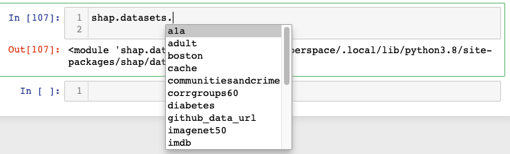
The shap library ships with some commonly used datasets, including the preprocessed version of the Adult Income Dataset used below.
Figure 1. Accessing datasets from the shap library
# create a train/test split

X_train, X_valid, y_train, y_valid = train_test_split(X, y, test_size=0.2, random_state=7)
Next, train an XGBoost model on the training data for 5K boosting rounds.
# read in the split dataset into an optimized data structure called Dmatrix required by XGBoost
dtrain = xgb.DMatrix(X_train, label=y_train)
dvalid = xgb.DMatrix(X_valid, label=y_valid)

%%time
# Feed the model the global bias
base_score = np.mean(y_train)
#Set hyperparameters for model training
params = {
   'objective': 'binary:logistic',
   'eval_metric': 'logloss',
   'eta': 0.01,
   'subsample': 0.5,
   'colsample_bytree': 0.8,
   'max_depth': 5,
   'base_score': base_score,
   'seed': SEED
}
# Train using early stopping on the validation dataset.
watchlist = [(dtrain, 'X_train'), (dvalid, 'X_test')]
model = xgb.train(params,
                       dtrain,
                       num_boost_round=5000,
                       evals=watchlist,
                       early_stopping_rounds=20,
                       verbose_eval=100)
===============================================================
Wall time: 14.3 s
The training execution takes 14.3 seconds on an Apple M1 8 Core CPU, with early stopping enabled.
See the XGBoost Parameters for more information on the configurable parameters within the XGBoost module.
Calculating SHAP values
SHAP comes in many different flavors depending on the nature of the algorithm. The most popular seem to be KernelSHAP, DeepSHAP, and TreeSHAP. While KernelSHAP is model-agnostic, TreeSHAP is only suitable for tree-based models (including the XGBoost model we just trained). Use the TreeExplainer class from the shap library to explain the entire dataset containing over 30K samples with over a thousand trees.
Using the same hardware outlined above, the SHAP values were calculated in 1.4 minutes. Note the timing to compare them with the values obtained in the next secNow that the SHAP values have been determined, the next step is interpretation. To understand the values, shap provides several different types of visualizations like force plots, summary plots, decision plots, and more, each highlighting a specific aspect of the model. Two plots are included below.
SHAP force plot
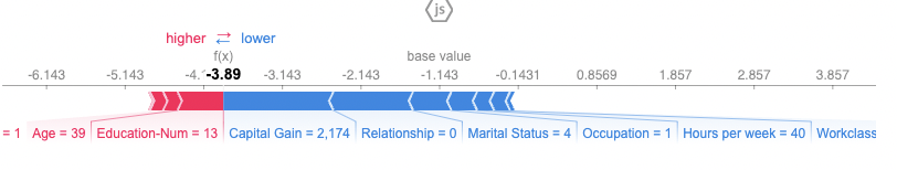
A force plot is used to explain a single instance in the dataset. Generate a force plot for the first row in the training set and see how the different features impact the prediction. First print the ground truth label and the model’s prediction for this data instance.
classes = {0 : 'False', 1: 'True'}

# ground truth label
y[0]
=========================
False

# Model Prediction
y_pred = [round(value) for value in model.predict(dvalid)]
classes[y_pred[0]]

==========================================================
False
The ground truth label for this person is False; that is, the person earns ≤$50K annually. The model also predicts the same. Figure 2 shows a force plot for the same person giving an insight into how the various features contributed towards the model’s prediction for this particular observation.
The base_value here is –1.143, while the target value for the selected sample is –3.89. All the values greater than the base value will have income ≥$50K and vice versa. For the chosen sample, the features appearing in red in Figure 2 push the prediction toward the base value while those in blue push the prediction away from the base value. It is therefore possible to infer that having a capital gain of 2,174 and relationship status of 0 negatively influences the model’s prediction for this particular person earning >$50K.
SHAP summary plot
The previous section looked at how SHAP was able to provide local explanations, or explanations specific to a single prediction. These values can be aggregated to get insights into a global view. A way to do this is by using theSHAP summary plots.
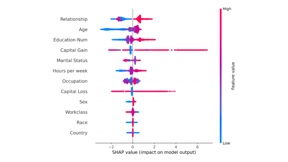
SHAP summary plots provide an overview of which features are more important for the model. This can be accomplished by plotting the SHAP values of every feature for every sample in the dataset. Figure 3 depicts a summary plot where each point in the graph corresponds to a single row in the dataset.
shap.summary_plot(shap_values_gpu, X_test)
Figure 3. SHAP summary plot
Each point in Figure 3 represents a row from the original dataset. For every point:
The y-axis indicates the features in order of importance from top to bottom. The x-axis refers to the actual SHAP values.
The horizontal location of a point represents the feature’s impact on the model’s prediction for that particular sample.
The color shows whether the value of a feature is high (red) or low (blue) for any row of the dataset.
From the summary plot, it is possible to infer that ‘Relationship status’ and ‘Age’ have a higher total model impact on predicting whether a person will earn a higher income or not, as compared to other features.
Step 2: GPU-accelerated SHAP
As discussed in the previous section, TreeSHAP is a version of SHAP tailored specifically for tree ensemble models. While TreeSHAP is relatively faster, it can also face typical computation issues when the ensemble size becomes too big. In such situations, taking advantage of the GPU acceleration is advisable to speed up the process.
However, the complexity of the TreeSHAP algorithm causes difficulty when mapping to hardware accelerators. This has led to the development of GPUTreeShap, a variation of the TreeSHAP algorithm suited to work with GPUs. It is now possible to take advantage of GPU hardware while computing SHAP values, thereby speeding up the entire model explanation process.
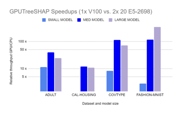
GPUTreeShap enables massively exact calculation of the shape values for tree-based algorithms. Figure 4 shows how GPUTreeSHAP provides an estimate of the gain achieved when using SHAP with GPU over CPU. According to GPUTreeShap: Massively Parallel Exact Calculation of SHAP Scores for Tree Ensembles, “With a single NVIDIA Tesla V100-32 GPU, we achieve speedups of up to 19x for SHAP values and speedups of up to 340x for SHAP interaction values over a state-of-the-art multi-core CPU implementation executed on two 20-core Xeon E5-2698 v4 2.2 GHz CPUs. We also experiment with multi-GPU computing using eight V100 GPUs, demonstrating throughput of 1.2M rows per second–equivalent CPU-based performance is estimated to require 6850 CPU cores.”
Figure 4. SHAP acceleration with GPU
Installation
GPUTreeShap already comes integrated with the Python shap package. Another way to access GPUTreeShap is by installing the RAPIDS data science framework. This ensures access to GPUTreeShap and a host of different libraries for executing end-to-end data science pipelines entirely in the GPU.
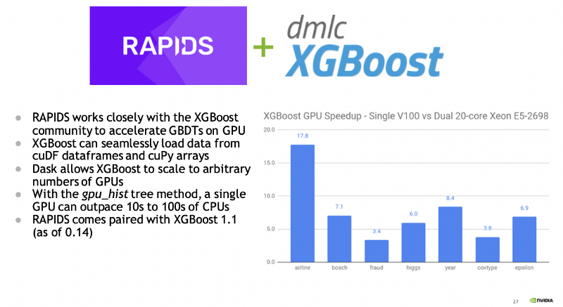
RAPIDS also comes integrated with XGBoost (as of 0.14). XGBoost was, in fact, the first popular ML Toolkit accelerated under what eventually became the RAPIDS ecosystem. Figure 5 highlights XGBoost speedup on GPU, comparing a single V100 GPU to a dual 20-core CPU.
Developers can take advantage of GPU acceleration for XGBoost and SHAP values with RAPIDS. The default open-source XGBoost packages already include GPU CUDA-capable GPUs support.
Figure 5. RAPIDS works closely with the XGBoost community to accelerate GBDTs on GPU
Training an XGBoost model with GPU acceleration
The previous section demonstrates who to train an XGBoost model on the Adult Income Dataset. This section repeats the same process enabled with GPU acceleration. This requires a change in the value of a single parameter called tree_method and delivers a massive decrease in the computation time.
Specify the tree_method parameter as gpu_hist, keeping all other parameters unchanged.
%%time
# Feed the model the global bias
base_score = np.mean(y_train)

#Set hyperparameters for model training
params = {
    'objective': 'binary:logistic',
    'eval_metric': 'logloss',
    'eta': 0.01,
    'subsample': 0.5,
    'colsample_bytree': 0.8,
    'max_depth': 5,
    'base_score': base_score,
    'tree_method': "gpu_hist", # GPU accelerated training
    'seed': SEED
}

# Train using early stopping on the validation dataset.
watchlist = [(dtrain, 'X_train'), (dvalid, 'X_test')]

model_gpu = xgb.train(params,
                        dtrain,
                        num_boost_round=5000,
                        evals=watchlist,
                        early_stopping_rounds=10,
                        verbose_eval=100)

=============================================================
CPU times: user 2.43 s, sys: 484 ms, total: 2.91 s
Wall time: 3.27 s
Training an XGBoost model with a single Tesla T4 GPU (available through Google Colab) helped in decreasing the training time from 14.3 seconds to just 3.27 seconds. A decrease in the compute time is beneficial since training machine learning models, especially on large datasets, can be both challenging and expensive.
Calculating SHAP values using GPU
When the GPU predictor is selected, XGBoost uses GPUTreeShap as a backend for computing shap values.
%%time
model_gpu.set_param({"predictor": "gpu_predictor"})
explainer_gpu = shap.TreeExplainer(model=model_gpu)
shap_values_gpu = explainer_gpu.shap_values(X)
==========================================================
CPU times: user 1.34 s, sys: 252 ms, total: 1.59 s
Wall time: 1.56 s
Using GPU, the computation time for calculating Shapley values decreases to 1.56 seconds, from 1.4 minutes, gaining a massive reduction in computation time. The gain would be even more prominent when the dataset involves millions of data points, which is typical in many industries.
Summary
Techniques like SHAP can make machine learning systems more trustworthy. If a model can be faithfully explained, it can be analyzed to determine whether it is fit to be deployed. This is an essential step toward inculcating trust in any technology. With GPU acceleration, it is possible to compute SHAP values faster, allowing you to gain insights into predictive models more quickly.
However, SHAP is not a silver bullet and has its own set of limitations.The main criticism of SHAP is that it can be misinterpreted. SHAP essentially helps in answering the question of why a particular observation received a prediction rather than a baseline value. This baseline value is dictated by the choice of a background dataset and can offer contrasting results if the reference dataset changes.
Consequently, the same observation can result in different SHAP values, depending on the choice of the background dataset. It is therefore important to carefully and appropriately choose background datasets keeping in mind the context of their use. It is important to understand the assumptions and trade-offs associated with explainability techniques in machine learning.

 On October 18, learn how to unlock one-third of AI compute on the NVIDIA Jetson AGX Orin by leveraging Deep Learning Accelerator for your embedded AI…
 This version 22.9 update to the NVIDIA HPC SDK includes fixes and minor enhancements.
 This self-paced, free tutorial provides a basic understanding of the NVIDIA Isaac Sim interface and the documentation needed to begin robot simulation projects.


 Extended reality, or XR, is a collective term that refers to immersive technologies, including virtual reality, augmented reality, and mixed reality.
 (2)") Machine learning (ML) is increasingly used across industries. Fraud detection, demand sensing, and credit underwriting are a few examples of specific use…
Machine learning (ML) is increasingly used across industries. Fraud detection, demand sensing, and credit underwriting are a few examples of specific use…