 Learn tools and techniques for accelerating C/C++ applications to run on massively parallel GPUs with CUDA.
Learn tools and techniques for accelerating C/C++ applications to run on massively parallel GPUs with CUDA.
 Learn tools and techniques for accelerating C/C++ applications to run on massively parallel GPUs with CUDA.
Learn tools and techniques for accelerating C/C++ applications to run on massively parallel GPUs with CUDA.
 Use of stolen or compromised credentials remains at the top of the list as the most common cause of a data breach. Because an attacker is using credentials or…
Use of stolen or compromised credentials remains at the top of the list as the most common cause of a data breach. Because an attacker is using credentials or passwords to compromise an organization’s network, they can bypass traditional security measures designed to keep adversaries out.
When they’re inside the network, attackers can move laterally and gain access to sensitive data, which can be extremely costly for an organization. In fact, it’s estimated that breaches caused by stolen or compromised credentials cost an average of $4.50 million in 2022.
Malicious activities in a network are hard to detect when performed by existing users, roles, or machine credentials. For this reason, these types of breaches take the longest, on average, to identify: 243 days and another 84 days on average to contain.
Companies might leverage user behavior analytics (UBA) to detect abnormal behavior based on a defined set of risks. With UBA, a baseline for each user or device is created and from that deviations from normal behaviors can be detected by comparing with past actions. UBA looks for patterns that might indicate anomalous behavior, based on known past behaviors.
There is an ever-increasing volume of data produced by a modern enterprise. Server logs, application logs, cloud logs, sensor telemetry, network, and disk information are now orders of magnitude larger than what can be stored by traditional security information and event management (SIEM) systems. The security operations team can examine only a fraction of that data.
Because enterprises are generating more data than they can collect and analyze, the vast majority of the data coming in goes untapped. Without tapping into this data, enterprises can’t build robust and rich models to enable them to detect deviations in their environment. The inability to examine this data leads to undetected security breaches, long remediation times, and ultimately huge financial issues for the company being breached.
But what if you could analyze 100% of the data across an enterprise—every user, every machine? People have unique characteristics and different ways that they interact with the network depending on their role. Understanding the day-to-day and moment-by-moment interactions of every user and device across the network is what we refer to as digital fingerprinting. Every user account within an organization has a unique digital fingerprint.
UBA looks for patterns that correlate bad behavior and focuses on threshold-based alerting. Digital fingerprinting is different because it identifies anti-patterns, or when things deviate from their normal patterns. For example, when a user account starts performing atypical yet permissible actions, traditional security methods may not trigger an alert.
To detect these anti-patterns, there must be a model for each user, to measure deviation. UBA is a shortcut because it tries to predict indicators of bad behavior. With digital fingerprinting, there are individual models to measure against.
To maximize the value of digital fingerprinting requires granularity and the ability to deploy thousands of models using unsupervised learning on a massive scale.
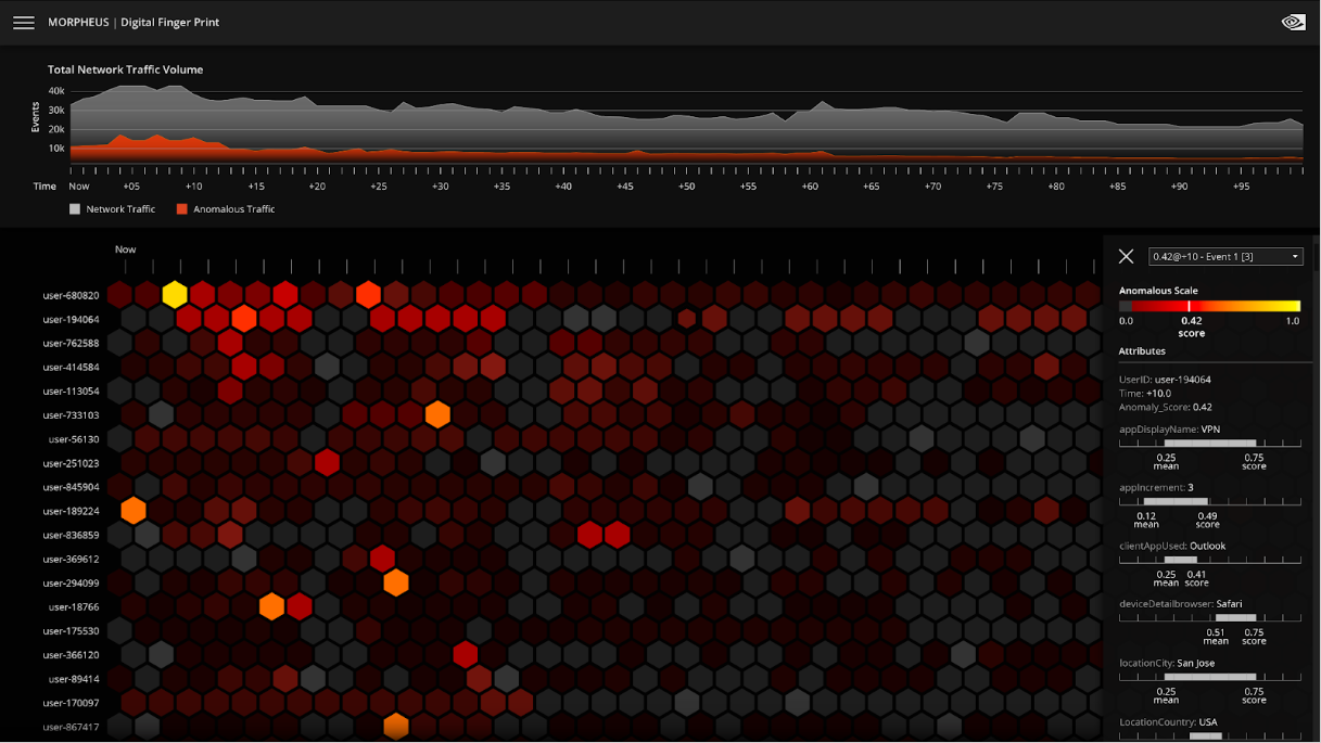
This can be done with NVIDIA Morpheus, a GPU-accelerated AI cybersecurity framework enabling developers to build optimized AI pipelines for filtering, processing, and classifying large volumes of real-time data. Morpheus includes a prebuilt, end-to-end workflow for digital fingerprinting, making it possible to achieve 100 percent data visibility.
A typical user may interact with 100 or more applications while doing their job. Integrations between these applications means that there may be tens of thousands of interconnections and permissions shared across those 100 applications. If you have 10,000 users, you’d need 10,000 models initially.
With the Morpheus digital fingerprinting pretrained workflow, massive amounts of data can be addressed, and hundreds of thousands, or even millions of models can be managed. Implementations of a digital fingerprinting workflow for cybersecurity enable organizations to analyze all the data across the network, as AI performs massive data filtration and reduction for real-time threat detection. Critical behavior anomalies can be rapidly identified for security analysts, so that they can more quickly identify and react to threats.
Experience the NVIDIA digital fingerprinting prebuilt model with a free hands-on lab on NVIDIA LaunchPad.
Julien Salinas wears many hats. He’s an entrepreneur, software developer and, until lately, a volunteer fireman in his mountain village an hour’s drive from Grenoble, a tech hub in southeast France. He’s nurturing a two-year old startup, NLP Cloud, that’s already profitable, employs about a dozen people and serves customers around the globe. It’s one Read article >
The post AI Esperanto: Large Language Models Read Data With NVIDIA Triton appeared first on NVIDIA Blog.
 NVIDIA JetPack provides a full development environment for hardware-accelerated AI-at-the-edge on Jetson platforms. Previously, a standalone version of NVIDIA…
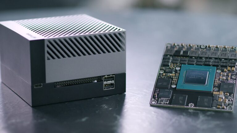
NVIDIA JetPack provides a full development environment for hardware-accelerated AI-at-the-edge on Jetson platforms. Previously, a standalone version of NVIDIA JetPack supports a single release of CUDA, and you did not have the ability to upgrade CUDA on a given NVIDIA JetPack version. NVIDIA JetPack is released on a rolling cadence with a single version of CUDA, typically being supported throughout each major release cycle (for example, NVIDIA JetPack 4.x or NVIDIA JetPack 5.x).
Starting with CUDA Toolkit 11.8, Jetson users on NVIDIA JetPack 5.0 and later can upgrade to the latest CUDA release without updating the NVIDIA JetPack version or Jetson Linux BSP (Board Support Package). You can stay on par with the CUDA Desktop releases.
To understand why the CUDA support model has been different between the desktop with discrete-GPU (dGPU) and Jetson with integrated-GPU (iGPU), it helps to understand the following:
Figure 1 shows the Jetson software architecture, with a core of the Jetson Linux BSP and layers of the various software components that make up the NVIDIA JetPack SDK. For more information, see Jetson Software Architecture.
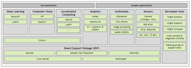
Figure 2 shows where CUDA resides in the overall NVIDIA JetPack SDK packaging structure and how it interacts with all other components of the Jetson Linux BSP. As you can see in Figure 2, the CUDA driver is part of the Jetson Linux BSP, along with other components. All these components update as per the release cadence and frequency of the Jetson Linux BSP, which has been different from the quarterly CUDA release cadence. The CUDA toolkit is separate from the BSP and does not package the CUDA driver.
When you install the NVIDIA JetPack SDK, the Jetson Linux BSP (containing the CUDA driver) and the CUDA toolkit get installed by default.
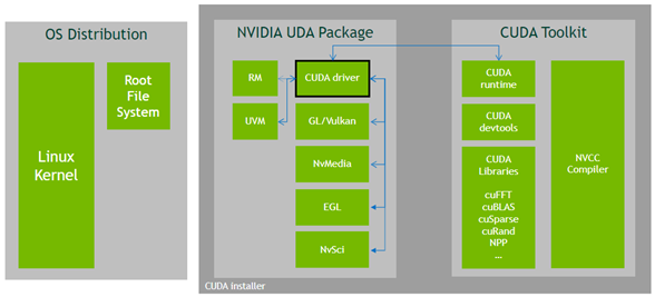
Due to this packaging structure, CUDA developers on desktop have the flexibility to stay up to date with the latest CUDA releases aligning with the CUDA quarterly release cadence. Moreover, features such as forward compatibility and minor version compatibility help you pick up combinations of driver and toolkit, and tailor it per your application needs.
Starting from CUDA 11.8, CUDA has introduced an upgrade path that provides Jetson developers with an option to update the CUDA driver and the CUDA toolkit to the latest versions.
Figure 4 shows blue boxes that depict components that are present by default in the NVIDIA JetPack 5.0 SDK. The dotted line separates Jetson Linux BSP from the other components that are part of the NVIDIA JetPack SDK. The green boxes indicate the CUDA components that you can upgrade to through this feature.
These upgrades are made possible by the introduction of the CUDA driver upgrade (also referred to as the CUDA compatibility package), as shown in Figure 5.
This upgrade package mainly contains the CUDA driver (libcuda.so.*) and its dependencies that enable you to access the latest and greatest CUDA functionalities that come with every quarterly CUDA release.
Without this package, you were previously limited to the functionality provided by the default CUDA driver that was packaged in the Jetson Linux BSP. You had no mechanism to upgrade to the latest CUDA driver and toolkit.
With this package, Jetson users who have invested in long and thorough validation cycles for the existing Jetson Linux BSP can upgrade to the latest CUDA versions. This upgrade is done over the existing Jetson Linux BSP, keeping it unchanged.
With CUDA 11.8, the CUDA Downloads page now displays a new architecture, aarch64-Jetson, as shown in Figure 6, with the associated aarch64-Jetson CUDA installer and provides step-by-step instructions on how to download and use the local installer, or CUDA network repositories, to install the latest CUDA release.
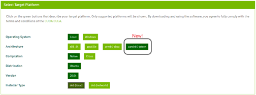
The new aarch64-Jetson CUDA installer packages both the CUDA Toolkit and the upgrade package together. The step-by-step installation instructions provided ensure that the CUDA upgrade package gets downloaded and installed along with the corresponding CUDA toolkit for Jetson devices.
The installed upgrade package is available in the versioned toolkit file directory. For example, you can find 11.8 in the following directory:
/usr/local/cuda-11.8/
The upgrade package consists of the following files:
libcuda.so.*: The CUDA driver.libnvidia-nvvm.so.*: Just-in-time link-time optimization (CUDA 11.8 and later only).libnvidia-ptxjitcompiler.so.*: The JIT (just-in-time) compiler for PTX files.These files together implement the CUDA driver interface. This package only provides the files and does not configure the system.
If you are working on an x86 host and cross-compiling to the aarch64-Jetson target, the U20.04 CUDA host installer can be found on the CUDA Downloads page. The cross-compile bits can be found in the following directory:
aarch64-jetson/cross/Ubuntu/20.04/deb installer
The following code example shows how the CUDA Upgrade package can be installed and used to run the applications.
$ sudo apt-get -y install cuda

Reading package lists...
Building dependency tree...
Reading state information...
The following additional packages will be installed:
  cuda-11-8 cuda-cccl-11-8 cuda-command-line-tools-11-8 cuda-compat-11-8
  ...…

The following NEW packages will be installed:
  cuda cuda-11-8 cuda-cccl-11-8 cuda-command-line-tools-11-8 cuda-compat-11-8
  ...…

0 upgraded, 48 newly installed, 0 to remove and 38 not upgraded.
Need to get 15.7 MB/1,294 MB of archives.
After this operation, 4,375 MB of additional disk space will be used.
Get:1 http://developer.download.nvidia.com/compute/cuda/repos/ubuntu2004/arm64  cuda-compat-11-8 11.8.31058490-1 [15.8 MB]
Fetched 15.7 MB in 12s (1,338 kB/s)
Selecting previously unselected package cuda-compat-11-8.
(Reading database ...
  ...…

(Reading database ... 100%
(Reading database ... 148682 files and directories currently installed.)
Preparing to unpack .../00-cuda-compat-11-8_11.8.31058490-1_arm64.deb ...
Unpacking cuda-compat-11-8 (11.8.31058490-1) ...
  ...…

Unpacking cuda-11-8 (11.8.0-1) ...
Selecting previously unselected package cuda.
Preparing to unpack .../47-cuda_11.8.0-1_arm64.deb ...
Unpacking cuda (11.8.0-1) ...
Setting up cuda-toolkit-config-common (11.8.56-1) ...
Setting up cuda-compat-11-8 (11.8.31058490-1) ...

$ ls -l /usr/local/cuda-11.8/compat
total 55300
lrwxrwxrwx 1 root root       12 Jan  6 19:14 libcuda.so -> libcuda.so.1
lrwxrwxrwx 1 root root       14 Jan  6 19:14 libcuda.so.1 -> libcuda.so.1.1
-rw-r--r-- 1 root root 21702832 Jan  6 19:14 libcuda.so.1.1
lrwxrwxrwx 1 root root       19 Jan  6 19:14 libnvidia-nvvm.so -> libnvidia-nvvm.so.4
lrwxrwxrwx 1 root root       23 Jan  6 19:14 libnvidia-nvvm.so.4 -> libnvidia-nvvm.so.4.0.0
-rw-r--r-- 1 root root 24255256 Jan  6 19:14 libnvidia-nvvm.so.4.0.0
-rw-r--r-- 1 root root 10665608 Jan  6 19:14 libnvidia-ptxjitcompiler.so
lrwxrwxrwx 1 root root       27 Jan  6 19:14 libnvidia-ptxjitcompiler.so.1 -> libnvidia-ptxjitcompiler.so

The user can set LD_LIBRARY_PATH to include the libraries installed by upgrade package before running the CUDA 11.8 application:
$ LD_LIBRARY_PATH=/usr/local/cuda-11.8/compat:$LD_LIBRARY_PATH ~/Samples/1_Utilities/deviceQuery
CUDA Device Query (Runtime API) version (CUDART static linking)
Detected 1 CUDA Capable device(s)
Device 0: "Orin"
  CUDA Driver Version / Runtime Version          11.8 / 11.8
  CUDA Capability Major/Minor version number:    8.7
      ......
deviceQuery, CUDA Driver = CUDART, CUDA Driver Version = 11.8, CUDA Runtime Version = 11.8, NumDevs = 1
Result = PASS
The default drivers (originally installed with NVIDIA JetPack and part of the Jetson Linux BSP) are retained by the installer. The application can use either the default version of CUDA (originally installed with NVIDIA JetPack) or the one installed by the upgrade package. Use the LD_LIBRARY_PATH variable to choose the required version.
Only a single CUDA upgrade package can be installed at any point in time on a given system. While installing a new CUDA upgrade package, the previous version of the installed upgrade package is removed and replaced with the new one. Installation of the upgrade package fails if it is not compatible with the NVIDIA JetPack version.
For example, applications that were previously compiled with CUDA 11.4 continue to work with the CUDA 11.8 upgrade package due to backward compatibility in the CUDA driver.
Table 1 shows the CUDA user-mode driver (UMD) and CUDA Toolkit version compatibility for the NVIDIA JetPack 5.0 release.
| CUDA UMD | CUDA Toolkit | |
| 11.4 (default; part of NVIDIA JetPack) |
11.8 | |
| 11.4 (default; part of NVIDIA JetPack) |
C | C (minor version compatibility) |
| 11.8 (with the upgrade package) |
C | C |
C = Compatible; X = Not compatible
On Jetson, the compute stack of CUDA, cuDNN, TensorRT, and so on, was tightly tied to a particular version of Jetson Linux (L4T). To upgrade to a newer version of the compute stack, you also had to deal with upgrading to Jetson Linux.
We are working towards a future where Jetson developers can migrate to newer versions of the compute libraries without upgrading Jetson Linux. This CUDA feature that enables upgrading CUDA is a step in that direction.
aarch64-Jetson and follow the installation instructions to upgrade your Jetson device to CUDA 11.8.Do register for the NVIDIA JetPack 5 deep-dive webinar. The CUDA and Jetson team walk you through details on this new feature and you get an opportunity to ask questions live!
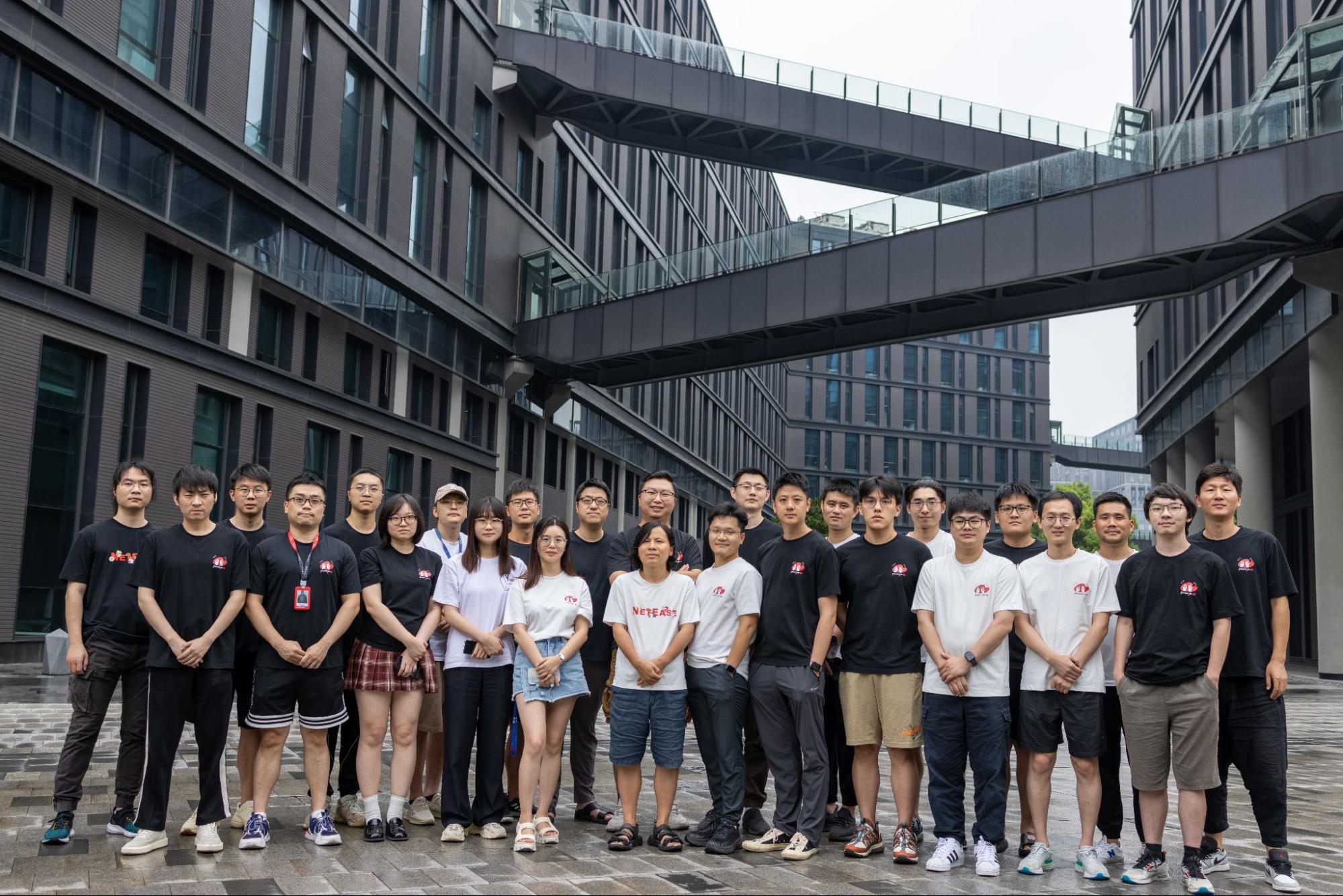
 We sat down with Dinggen Zhan of NetEase to discuss his team’s implementation of path tracing in the popular martial arts game, Justice Online. What is your…
We sat down with Dinggen Zhan of NetEase to discuss his team’s implementation of path tracing in the popular martial arts game, Justice Online.
What is your professional background and current job role?
I have more than 20 years of experience in the gaming industry. I joined NetEase in 2012, and am now senior technical expert and lead programmer for Justice.
Why did NetEase decide to integrate a path tracer into Justice?
Back in 2018, NVIDIA launched the first RTX GPU. At that time, we immediately integrated RTX features into Justice and quickly pushed it online. NVIDIA RTX Path Tracing is the ultimate solution for ray tracing. It has excellent visual results and solves all the pain points caused by illumination under rasterization. We stick to using cutting-edge technologies in our development work to create high-image quality games and enhance players’ immersive gaming experience.
What NVIDIA technologies did you use to make the path tracing work?
We used DLSS 3, Real-time Denoisers (NRD), Reflex, and Restir GI.
How did the path tracer affect your lighting production during the Justice development process?
The path tracing technology provides a way to create realistic illumination systems, especially suitable for producing natural and delicate indirect illuminations. Therefore, we do not need to spend time manually adjusting lights in scenes. Instead, we only need to add the corresponding lights for emissive objects such as lanterns and leave the rest to the path tracer to complete the calculation.
Why is physically accurate lighting important for the games you develop?
The rendering pipeline of Justice is built on physically based rendering (PBR). Realistic physical illumination is naturally implemented with path tracing, which improves visual appeal and reduces defects. The artists have more control over the look, and it is convenient to integrate.
What challenges did you face during the process of integrating ray tracing?
New technologies generally bring new problems, and the debugging process is particularly more difficult. Fortunately, NVIDIA has upgraded the NVIDIA Nsight debugging tool in time, making it an easier process for development work. The current real-time path tracer needs to be improved over several optical effects including caustics, translucency, and the skin materials of subsurface scattering.

What challenges were you looking to solve with the path tracer?
In the past, rasterized rendering of direct illumination, indirect illumination, reflection, and shadow were done with separated passes, which could not ensure accuracy. Path tracing unifies the computation of light transport, simplifies the whole rendering pipeline, and makes the final results immediately visible, allowing artists more control for content creation.
How long did it take for you to get the path tracer up and running?
From beginning to end, it took us about five to six months. The first three months were mainly for function integration, while the later stage was focused on effect tuning, performance optimization, and debugging.
Did you encounter any surprises during the integration process?
The realism of the path-traced pictures is amazing, and one notch above basic ray tracing. NVIDIA DLSS 3 also boosts the performance of the path tracer beyond all expectations.
How has path tracing affected your visuals and gameplay?
Path tracing can help game visuals reach cinematic realism, bringing the real-time rendering experience to the film production level. Video game players will feel like they are in the real world of each game. The visual experience is unprecedented, and there are infinite possibilities for the current metaverse development.

Can you share any tips or lessons learned for other developers looking to integrate path tracing technology?
First, make sure that your game engine has a physically based rendering pipeline, which will reduce the integration issues. For certain special materials, the current path tracer cannot work completely without rasterization, and it is recommended to use in conjunction with a rasterizer.
Second, pay attention to the coherence of motion vectors and depth because the denoiser is quite sensitive to motion vectors, whether the motion vectors are in world space or screen space. The flag settings of the denoiser must be correct too. The depth buffer is in the floating-point range (0-1), and if it is reversed, it can affect the denoising and anti-aliasing results.
Third, our path tracing is based on the NVIDIA Falcor engine, which is written in the shader language Slang. Integrating is a complicated and time-consuming task. We chose to translate Slang into HLSL at first. Since manually translating the entire Falcor shaders could be an onerous task, we simplified the Falcor codebase. Debugging costs us significant time. Looking back now, it would have been wise to take time to support the entire Slang at the beginning of the integration and put in the whole Falcor path tracing codebase. The integration process might go smoother, save us some time, and help support Falcor’s future functionalities and features.
Do you plan to integrate path tracing into future NetEase games?
The amazing visual quality of path tracing is beyond the reach of any rasterization technique. In the future, we will continue investing more resources to develop path traced levels, and improve the quality and performance in the game.
Visit the NetEase website for more information about the company.
Learn more about the NVIDIA RTX Path Tracing SDK, and sign up to be notified when it is publicly available. For more resources, visit NVIDIA Game Development.
Frame interpolation is the process of synthesizing in-between images from a given set of images. The technique is often used for temporal up-sampling to increase the refresh rate of videos or to create slow motion effects. Nowadays, with digital cameras and smartphones, we often take several photos within a few seconds to capture the best picture. Interpolating between these “near-duplicate” photos can lead to engaging videos that reveal scene motion, often delivering an even more pleasing sense of the moment than the original photos.
Frame interpolation between consecutive video frames, which often have small motion, has been studied extensively. Unlike videos, however, the temporal spacing between near-duplicate photos can be several seconds, with commensurately large in-between motion, which is a major failing point of existing frame interpolation methods. Recent methods attempt to handle large motion by training on datasets with extreme motion, albeit with limited effectiveness on smaller motions.
In “FILM: Frame Interpolation for Large Motion”, published at ECCV 2022, we present a method to create high quality slow-motion videos from near-duplicate photos. FILM is a new neural network architecture that achieves state-of-the-art results in large motion, while also handling smaller motions well.
 |
| FILM interpolating between two near-duplicate photos to create a slow motion video. |
FILM Model Overview
The FILM model takes two images as input and outputs a middle image. At inference time, we recursively invoke the model to output in-between images. FILM has three components: (1) A feature extractor that summarizes each input image with deep multi-scale (pyramid) features; (2) a bi-directional motion estimator that computes pixel-wise motion (i.e., flows) at each pyramid level; and (3) a fusion module that outputs the final interpolated image. We train FILM on regular video frame triplets, with the middle frame serving as the ground-truth for supervision.
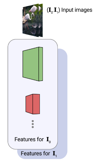 |
| A standard feature pyramid extraction on two input images. Features are processed at each level by a series of convolutions, which are then downsampled to half the spatial resolution and passed as input to the deeper level. |
Scale-Agnostic Feature Extraction
Large motion is typically handled with hierarchical motion estimation using multi-resolution feature pyramids (shown above). However, this method struggles with small and fast-moving objects because they can disappear at the deepest pyramid levels. In addition, there are far fewer available pixels to derive supervision at the deepest level.
To overcome these limitations, we adopt a feature extractor that shares weights across scales to create a “scale-agnostic” feature pyramid. This feature extractor (1) allows the use of a shared motion estimator across pyramid levels (next section) by equating large motion at shallow levels with small motion at deeper levels, and (2) creates a compact network with fewer weights.
Specifically, given two input images, we first create an image pyramid by successively downsampling each image. Next, we use a shared U-Net convolutional encoder to extract a smaller feature pyramid from each image pyramid level (columns in the figure below). As the third and final step, we construct a scale-agnostic feature pyramid by horizontally concatenating features from different convolution layers that have the same spatial dimensions. Note that from the third level onwards, the feature stack is constructed with the same set of shared convolution weights (shown in the same color). This ensures that all features are similar, which allows us to continue to share weights in the subsequent motion estimator. The figure below depicts this process using four pyramid levels, but in practice, we use seven.
Bi-directional Flow Estimation
After feature extraction, FILM performs pyramid-based residual flow estimation to compute the flows from the yet-to-be-predicted middle image to the two inputs. The flow estimation is done once for each input, starting from the deepest level, using a stack of convolutions. We estimate the flow at a given level by adding a residual correction to the upsampled estimate from the next deeper level. This approach takes the following as its input: (1) the features from the first input at that level, and (2) the features of the second input after it is warped with the upsampled estimate. The same convolution weights are shared across all levels, except for the two finest levels.
Shared weights allow the interpretation of small motions at deeper levels to be the same as large motions at shallow levels, boosting the number of pixels available for large motion supervision. Additionally, shared weights not only enable the training of powerful models that may reach a higher peak signal-to-noise ratio (PSNR), but are also needed to enable models to fit into GPU memory for practical applications.
 |
 |
| The impact of weight sharing on image quality. Left: no sharing, Right: sharing. For this ablation we used a smaller version of our model (called FILM-med in the paper) because the full model without weight sharing would diverge as the regularization benefit of weight sharing was lost. |
Fusion and Frame Generation
Once the bi-directional flows are estimated, we warp the two feature pyramids into alignment. We obtain a concatenated feature pyramid by stacking, at each pyramid level, the two aligned feature maps, the bi-directional flows and the input images. Finally, a U-Net decoder synthesizes the interpolated output image from the aligned and stacked feature pyramid.
Loss Functions
During training, we supervise FILM by combining three losses. First, we use the absolute L1 difference between the predicted and ground-truth frames to capture the motion between input images. However, this produces blurry images when used alone. Second, we use perceptual loss to improve image fidelity. This minimizes the L1 difference between the ImageNet pre-trained VGG-19 features extracted from the predicted and ground truth frames. Third, we use Style loss to minimize the L2 difference between the Gram matrix of the ImageNet pre-trained VGG-19 features. The Style loss enables the network to produce sharp images and realistic inpaintings of large pre-occluded regions. Finally, the losses are combined with weights empirically selected such that each loss contributes equally to the total loss.
Shown below, the combined loss greatly improves sharpness and image fidelity when compared to training FILM with L1 loss and VGG losses. The combined loss maintains the sharpness of the tree leaves.
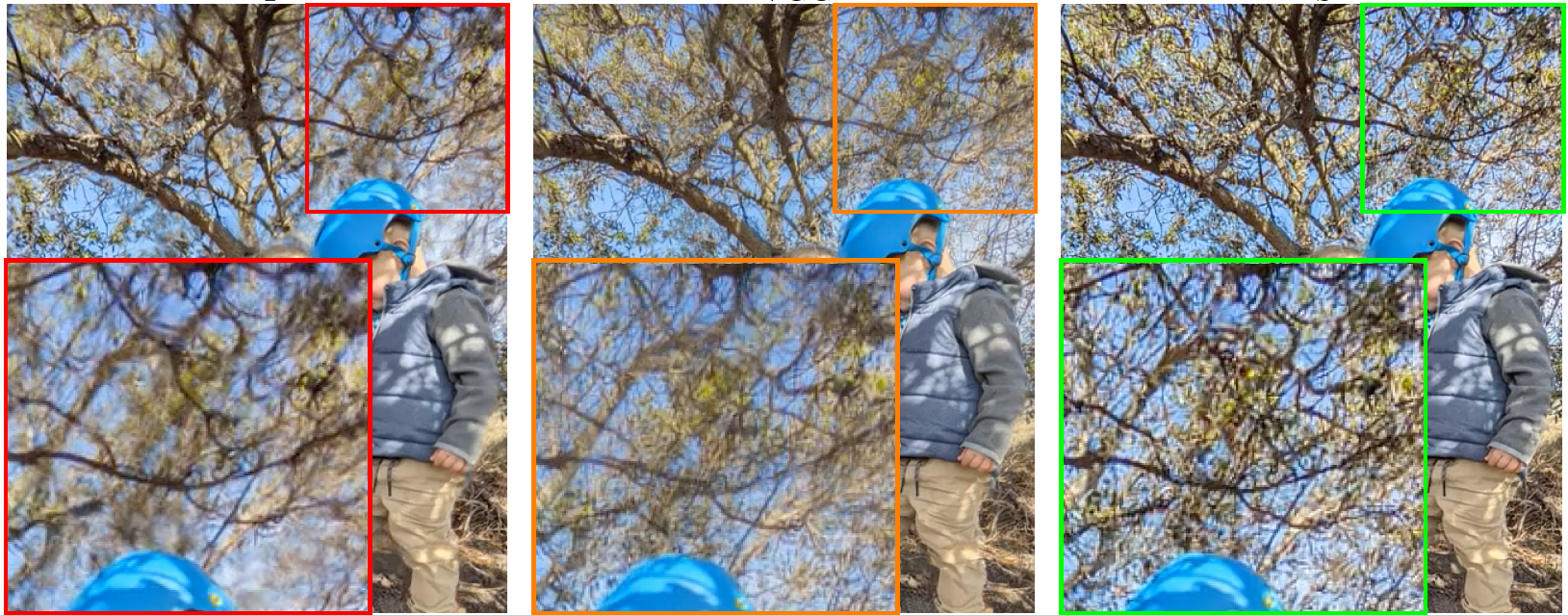 |
| FILM’s combined loss functions. L1 loss (left), L1 plus VGG loss (middle), and Style loss (right), showing significant sharpness improvements (green box). |
Image and Video Results
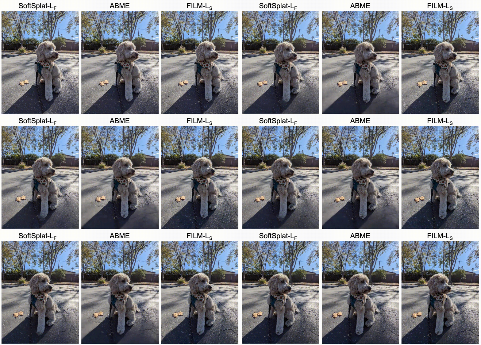
We evaluate FILM on an internal near-duplicate photos dataset that exhibits large scene motion. Additionally, we compare FILM to recent frame interpolation methods: SoftSplat and ABME. FILM performs favorably when interpolating across large motion. Even in the presence of motion as large as 100 pixels, FILM generates sharp images consistent with the inputs.
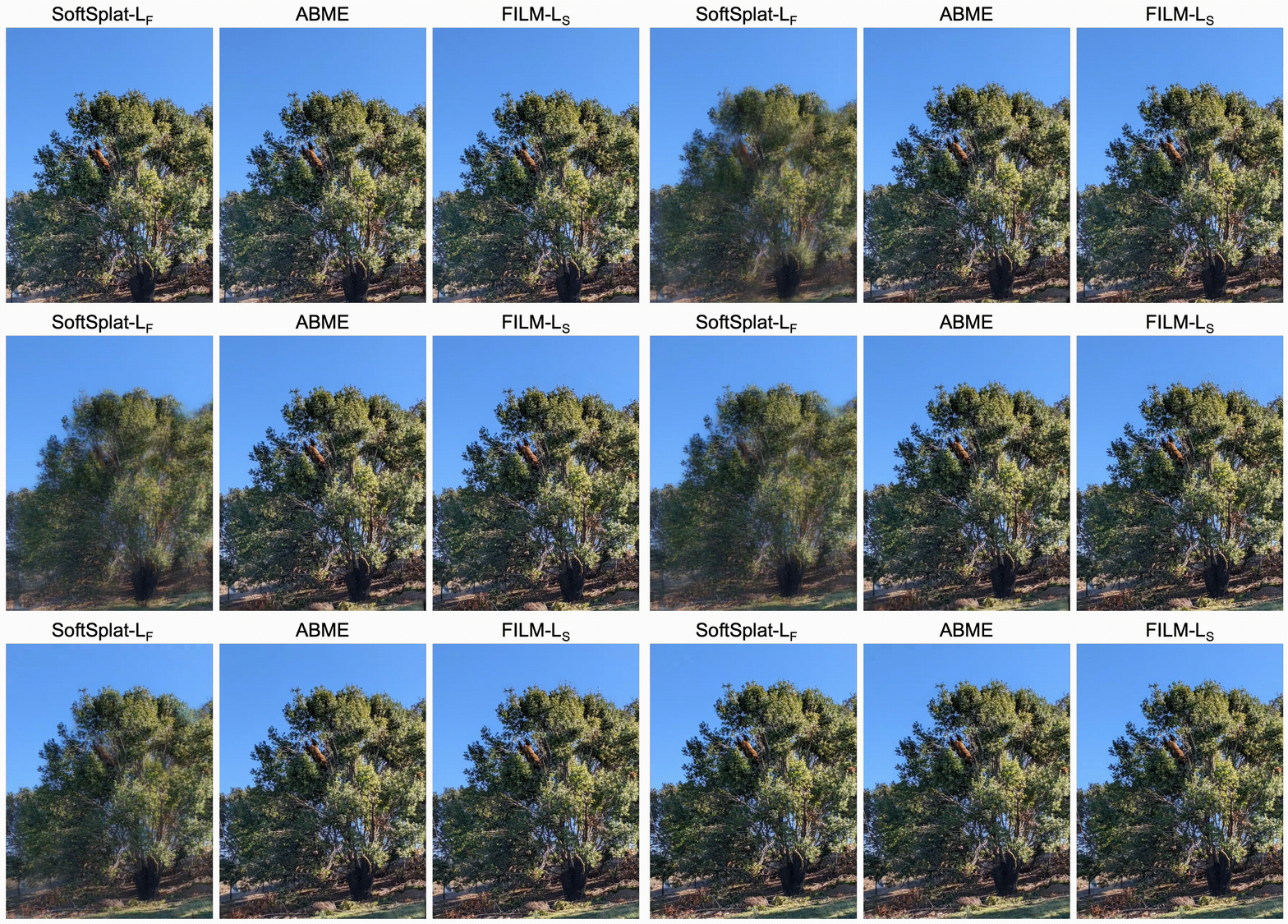 |
| Frame interpolation with SoftSplat (left), ABME (middle) and FILM (right) showing favorable image quality and temporal consistency. |
 |
Conclusion
We introduce FILM, a large motion frame interpolation neural network. At its core, FILM adopts a scale-agnostic feature pyramid that shares weights across scales, which allows us to build a “scale-agnostic” bi-directional motion estimator that learns from frames with normal motion and generalizes well to frames with large motion. To handle wide disocclusions caused by large scene motion, we supervise FILM by matching the Gram matrix of ImageNet pre-trained VGG-19 features, which results in realistic inpainting and crisp images. FILM performs favorably on large motion, while also handling small and medium motions well, and generates temporally smooth high quality videos.
Try It Out Yourself
You can try out FILM on your photos using the source codes, which are now publicly available.
Acknowledgements
We would like to thank Eric Tabellion, Deqing Sun, Caroline Pantofaru, Brian Curless for their contributions. We thank Marc Comino Trinidad for his contributions on the scale-agnostic feature extractor, Orly Liba and Charles Herrmann for feedback on the text, Jamie Aspinall for the imagery in the paper, Dominik Kaeser, Yael Pritch, Michael Nechyba, William T. Freeman, David Salesin, Catherine Wah, and Ira Kemelmacher-Shlizerman for support.
 NVIDIA announces the newest CUDA Toolkit software release, 11.8. This release is focused on enhancing the programming model and CUDA application speedup through…
NVIDIA announces the newest CUDA Toolkit software release, 11.8. This release is focused on enhancing the programming model and CUDA application speedup through new hardware capabilities.
New architecture-specific features in NVIDIA Hopper and Ada Lovelace are initially being exposed through libraries and framework enhancements. The full programming model enhancements for the NVIDIA Hopper architecture will be released starting with the CUDA Toolkit 12 family.
CUDA 11.8 has several important features. This post offers an overview of the key capabilities.
CUDA applications can immediately benefit from increased streaming multiprocessor (SM) counts, higher memory bandwidth, and higher clock rates in new GPU families.
CUDA and CUDA libraries expose new performance optimizations based on GPU hardware architecture enhancements.
Building on the lazy kernel loading feature in 11.7, NVIDIA added lazy loading to the CPU module side. What this means is that functions and libraries load faster on the CPU, with sometimes substantial memory footprint reductions. The tradeoff is a minimal amount of latency at the point in the application where the functions are first loaded. This is lower overall than the total latency without lazy loading.
All libraries used with lazy loading must be built with 11.7+ to be eligible for lazy loading.
Lazy loading is not enabled in the CUDA stack by default in this release. To evaluate it for your application, run with the environment variable CUDA_MODULE_LOADING=LAZY set.
You can now terminate with SIGINT or SIGKILL any applications running in MPS environments without affecting other running processes. While not true error isolation, this enhancement enables more fine-grained application control, especially in bare-metal data center environments.
NVIDIA JetPack provides a full development environment for hardware-accelerated AI-at-the-edge on Jetson platforms. Starting from CUDA Toolkit 11.8, Jetson users on NVIDIA JetPack 5.0 and later can upgrade to the latest CUDA versions without updating the NVIDIA JetPack version or Jetson Linux BSP (board support package) to stay on par with the CUDA desktop releases.
For more information, see Simplifying CUDA Upgrades for NVIDIA Jetson Developers.
Compute developer tools are designed in lockstep with the CUDA ecosystem to help you identify and correct performance issues.
In Nsight Compute, you can expose low-level performance metrics, debug API calls, and visualize workloads to help optimize CUDA kernels. New compute features are being introduced in CUDA 11.8 to aid performance tuning activity on the NVIDIA Hopper architecture.
You can now profile and debug NVIDIA Hopper thread block clusters, which provide performance boosts and increased control over the GPU. Cluster tuning is being released in combination with profiling support for the Tensor Memory Accelerator (TMA), the NVIDIA Hopper rapid data transfer system between global and shared memory.
A new sample is included in Nsight Compute for CUDA 11.8 as well. The sample provides source code and precollected results that walk you through an entire workflow to identify and fix an uncoalesced memory access problem. Explore more CUDA samples to equip yourself with the knowledge to use toolkit features and solve similar cases in your own application.
Profiling with Nsight Systems can provide insight into issues such as GPU starvation, unnecessary GPU synchronization, insufficient CPU parallelizing, and expensive algorithms across the CPUs and GPUs. Understanding these behaviors and the load of deep learning frameworks, such as PyTorch and TensorFlow, helps you tune your models and parameters to increase overall single or multi-GPU utilization.
Also included in the CUDA toolkit, both CUDA-GDB for CPU and GPU thread debugging as well as Compute Sanitizer for functional correctness checking have support for the NVIDIA Hopper architecture.
This release of the CUDA 11.8 Toolkit has the following features:
For more information, see the following resources:
Planes taxiing for long periods due to ground traffic — or circling the airport while awaiting clearance to land — don’t just make travelers impatient. They burn fuel unnecessarily, harming the environment and adding to airlines’ costs. Searidge Technologies, based in Ottawa, Canada, has created AI-powered software to help the aviation industry avoid such issues, Read article >
The post Searidge Technologies Offers a Safety Net for Airports appeared first on NVIDIA Blog.
TwitchCon — the world’s top gathering of live streamers – kicks off Friday with the new line of GeForce RTX 40 Series GPUs bringing incredible new technology — from AV1 to AI — to elevate live streams for aspiring and professional Twitch creators alike.
The post Creator EposVox Shares Streaming Lessons, Successes This Week ‘In the NVIDIA Studio’ appeared first on NVIDIA Blog.
 Fraud is a major problem for many financial services firms, costing billions of dollars each year, according to a recent Federal Trade Commission report….
Fraud is a major problem for many financial services firms, costing billions of dollars each year, according to a recent Federal Trade Commission report. Financial fraud, fake reviews, bot assaults, account takeovers, and spam are all examples of online fraud and harmful activity.
Although these firms employ techniques to combat online fraud, the methods can have severe limitations. Simple rule-based techniques and feature-based algorithm techniques (logistic regression, Bayesian belief networks, CART, and others) aren’t adaptable enough to detect the full range of fraudulent or suspicious online behaviors.
Fraudsters, for example, might set up many coordinated accounts to avoid triggering limitations on individual accounts. In addition, detecting fraudulent behavior patterns at scale is difficult due to the huge volume of data to sift through (billions of rows, tens of terabytes), the complexity of continually improving methodologies, and the scarcity of real cases of fraudulent activity required for training classification algorithms. For more details, see Intelligent Financial Fraud Detection Practices: An Investigation.
Although the cost of fraud is billions of dollars per year, there are very few fraudulent transactions among many legitimate transactions, leading to an imbalance in labeled data, when it is even available. Detecting fraud becomes even more complex in the financial services industry, due to security concerns around personal data and the need for transparency in the methods used to detect the fraudulent activity.
An explainable model enables fraud analysts to understand what inputs the algorithm used in the analysis and the reason(s) for flagging the transaction, building a stronger trust in the system. Additional benefits include the ability to communicate feedback to internal teams and provide customers with an explanation.
In recent years, graph neural networks (GNNs) have gained traction for fraud detection problems, revealing suspicious nodes (in accounts and transactions, for example) by aggregating their neighborhood information through different relations. In other words, by checking whether a given account has sent a transaction to a suspicious account in the past.
In the context of fraud detection, the ability of GNNs to aggregate information contained within the local neighborhood of a transaction enables them to identify larger patterns that may be missed by just looking at a single transaction.
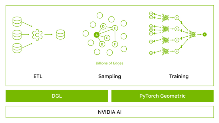
To enable developers to quickly take advantage of GNNs to optimize and accelerate fraud detection, NVIDIA partnered with the Deep Graph Library (DGL) team and the PyTorch Geometric (PyG) team to provide a GNN framework containerized solution that includes the latest DGL or PyG, PyTorch, NVIDIA RAPIDS, and a set of tested dependencies. The NVIDIA-optimized GNN Framework containers are performance-tuned and tested for NVIDIA GPUs.
This approach eliminates the need to manage packages and dependencies or build the framework from source. We are actively contributing to enhance the performance of these top GNN frameworks. We have added GPU support for unified virtual addressing (UVA), FP16 operations, neighborhood sampling, subgraph operations for minibatches and optimized sparse embeddings, sparse adam optimizer, graph batching, CSR-to-COO conversions, and much more.
This post first addresses the unique problems in credit card fraud detection and the most widely used detection techniques. It also highlights how GNNs accelerated by GPUs have a unique approach to addressing these issues. We walk through an end-to-end workflow showcasing best practices for preprocessing, training, and deployment for detecting fraud on a financial fraud dataset using graph neural networks. Last, we show benchmarks of end-to-end workflows on two industry scale datasets utilizing the optimizations contributed in DGL by NVIDIA engineers.
Fraud detection is a set of processes and analyses that allow firms to identify and prevent unauthorized activity. It has become one of the major challenges for most organizations, particularly those in banking, finance, retail, and e-commerce.
Any kind of fraud negatively affects an organization’s bottom line and market reputation, and deters both future prospects and current customers. Given the scale and reach of these vulnerable organizations, it has become crucial for them to prevent fraud from happening and even predict suspicious actions in real time.
Fraud detection poses unique problems for machine learning researchers and engineers, a few of which are detailed below.
Fraudsters update their knowledge and develop sophisticated techniques to cheat the system, often involving complex chains of transactions to avoid detection.
Traditional ruled-based systems and tabular machine learning (ML) like SVMs and XGBoost often can only consider the immediate edges of a transaction (who sent money to who), often missing patterns of fraud with more complex context. Rule-based systems also need to be hand-tuned over time as patterns of fraud change and new exploits emerge.
Available fraud datasets are often both imbalanced and without exhaustive labels. In the real world, only a small percentage of people intend to commit fraud. Domain experts typically classify transactions as either fraudulent or not, but cannot guarantee that all fraud has been captured in the dataset.
This class imbalance and lack of exhaustive labels make it difficult to develop supervised models, as models trained on the labels we do have may incur higher rates of false negatives, and the imbalanced dataset can lead to models that also generate more false positives. Thus, training GNNs with alternative objectives and using their latent representations downstream can have beneficial effects.
Predicting whether a transaction is fraudulent or not is not sufficient for transparency expectations in the financial services industry. It is also necessary to understand why certain transactions are flagged as fraud. This explanabity is important for understanding how fraud happens, how to implement policies to reduce fraud, and to make sure the process isn’t biased. Therefore, fraud detection models are required to be interpretable and explainable which limits the selection of models that analysts can use.
A series of transactions can be accurately described as a graph, with users being represented as nodes, and transactions between them being represented as edges. While feature-based algorithms like XGBoost and deep feature-based models like DLRM focus on the features of a single node or edge, graph-based approaches can take the features and structure of the local graph context (neighbors and neighbors of neighbors, for example) into account in their predictions.
In the traditional (non-GNN) graph domain, there are many approaches to generating salient predictions based on the graph structure. Statistical approaches that aggregate features from adjacent neighboring nodes or edges, or even their neighbors, can be used to provide information about locality to feature-based tabular algorithms like XGBoost.
Algorithms like the Louvain method and InfoMap can detect communities and denser clusters of users on the graph, which can then be used to detect communities and generate features that represent graph structure as a hierarchy.
While these approaches can generate adequate results, the problem remains that the algorithms used lack expressivity with respect to the graph itself, as they do not consider the graph in its native format.
Graph neural networks build on the concept of representing local structural and feature context natively within the model. Information from both edge and node features is propagated through aggregation and message passing to neighboring nodes.
When multiple layers of graph convolution are performed, this results in a node’s state containing some information from nodes multiple layers away, effectively allowing the GNN to have a “receptive field” of nodes or edges multiple jumps away from the node or edge in question.
In the context of the fraud detection problem, this large receptive field of GNNs can account for more complex or longer chains of transactions that fraudsters can use for obfuscation. Additionally, changing patterns can be accounted for by iterative retraining of the model.
Graph neural networks also benefit from being able to encode meaningful representations of nodes or edges while training on an unsupervised or self-supervised task, such as Bootstrapped Graph Latents (BGRL) or link prediction with negative sampling. This allows GNN users to pre-train a model without labels, and to fine-tune the model on the much sparser labels later in the pipeline, or to output strong representations of the graph. The representation output can be used for downstream models like XGBoost, other GNNs, or clustering techniques.
GNNs also have a suite of tools to enable explainability with respect to the input graph. Certain GNN models like heterogeneous graph transformer (HGT) and graph attention network (GAT) enable an attention mechanism across the adjacent edges of a node at each layer of the GNN, allowing the user to identify the path of messages that the GNN is using to derive its final state. Even if GNN models have no attention mechanism, a variety of approaches have been proposed in order to explain GNN output in the context of the entire subgraph, including GNNExplainer, PGExplainer, and GraphMask.
The next section walks through an end-to-end credit card fraud detection workflow. This workflow uses TabFormer, a card transaction fraud dataset, and trains a R-GCN (relational graph convolutional network) model on a variation of the link prediction task in order to generate enriched node embeddings. These node embeddings are passed to a downstream XGBoost model which is trained and subsequently performs fraud detection.
This XGBoost model can then be easily deployed. The embeddings trained can subsequently be used for other unsupervised techniques like clustering to identify undiscovered patterns of use without needing labels. Last, we will show benchmarks of end-to-end workflows on two industry scale datasets utilizing the optimizations contributed in DGL by NVIDIA engineers.
We are using the Tabformer dataset provided by IBM to demonstrate this workflow. The TabFormer dataset is a synthetic close approximation of a real-world financial fraud-detection dataset, consisting of:
To begin, preprocess the dataset using a predefined workflow. The workflow leverages cuDF, a GPU DataFrame library, to perform feature transformations on the original dataset to prepare it for graph construction. cuDF is a drop in replacement of pandas that enables the preprocessing of data directly on GPUs.
In this dataset, the card_id is defined as one card by one user. A specific user can have multiple cards, which would correspond to multiple different card_ids for this graph. The merchant_id is the categorical encoding of the feature, ‘Merchant Name’. The data is split such that the training data is all transactions before the year 2018, the validation data is all transactions during the year 2018, and the test data is all transactions after the year 2018.
# Read the dataset
data = cudf.read_csv(self.source_path)
data[“card_id”] = data[“user”].astype(“str”) + data[“card”].astype(“str”)

# Split the data based on the year
data["split"] = cudf.Series(np.zeros(data["year"].size), dtype=np.int8)
data.loc[data["year"] == 2018, "split"] = 1
data.loc[data["year"] > 2018, "split"] = 2
train_card_id = data.loc[data["split"] == 0, "card_id"]
train_merch_id = data.loc[data["split"] == 0, "merchant_id"]
Strip the ‘$’ from the ‘Amount’ to cast that value as a float. Keep card_id and merchant_id in the validation and test datasets only if they are included in the train datasets.
The graph is constructed with transaction edges between card_id and merchant_id.
Further preprocessing includes one hot encoding the Use chip feature, label encoding the ‘Is Fraud?’ feature, and target encoding the categorical representations of Merchant State, Merchant City, Zip, and MCC. In addition, the possible values of ‘Errors?’ are one hot encoded.
# Target encoding
high_card_cols = ["merchant_city", "merchant_state", "zip", "mcc"]
for col in high_card_cols:
    tgt_encoder = TargetEncoder(smooth=0.001)
    train_df[col] = tgt_encoder.fit_transform(
        train_df[col], train_df["is_fraud"])
    valtest_df[col] = tgt_encoder.transform(valtest_df[col])

# One hot encoding `use_chip`
oneh_enc_cols = ["use_chip"]
data = cudf.concat([data, cudf.get_dummies(data[oneh_enc_cols])], axis=1)

# Label encoding `is_fraud`
label_encoder = LabelEncoder()
train_df["is_fraud"] = label_encoder.fit_transform(train_df["is_fraud"])
valtest_df["is_fraud"] = label_encoder.transform(valtest_df["is_fraud"])

# One hot encoding the errors
exploded = data["errors"].str.strip(",").str.split(",").explode()
raw_one_hot = cudf.get_dummies(exploded, columns=["errors"])
errs = raw_one_hot.groupby(raw_one_hot.index).sum()
Once the dataset is preprocessed, transform the tabular format of the dataset into a graph.
Transforming a table (or multiple tables) into a graph centers around mapping the existing table(s) into the edges, nodes, and features for both structures. In the case of this dataset, we begin by using the transaction table to create edges between the cards and the merchants. In contemporary GNN frameworks, graph edges are represented at a basic level by pairs of node IDs. Nodes are implicit based on the IDs included in the edge lists.
# Defining node type
for ntype in ["card", "merchant"]:
   node_type = {MetadataKeys.NAME: ntype, MetadataKeys.FEAT: []}
   self.node_types.append(node_type)

# Adding attributes of edge data
self.edge_data = dict()
self.edge_data["transaction"] = cudf.DataFrame({
  MetadataKeys.SRC_ID: data["card_id"],
  MetadataKeys.DST_ID: data["merchant_id"],})

# Defining features
features = []
for key in data.keys():
  if key not in ["card_id", "merchant_id"]:
    self.edge_data["transaction"][key] = data[key]
      feat = {
       MetadataKeys.NAME: key,
       MetadataKeys.DTYPE: str(self.edge_data["transaction"][key].dtype),
       MetadataKeys.SHAPE: self.edge_data["transaction"][key].shape,}
      if key in ["is_fraud"]:
        feat[MetadataKeys.LABEL] = True
      features.append(feat)
With the base graph created, it’s time to add the transaction features onto the edges in the graph. Note that in this case, the transaction data is only edge-specific, so the output graph has no node features.
Once the graph is created and populated with features, the model can be applied to it.
Given the label imbalance and imperfect labeling of the dataset, we elected to use an unsupervised task, link prediction, to train the model to create meaningful representations of the nodes. The objective of link prediction is to predict the probability that an edge exists between two nodes. In financial services, this is translated to predicting the probability that a transaction exists between an individual and a merchant.
Some target nodes within the batch are true edges, which are actual edges that exist in the graph, while others, generated by a negative sampler, are negative edges that do not truly exist. Negative edges are necessary in this case because our training task is the classification between real and fake. There are a variety of proposed ways in which to generate negative edges, but simply uniformly sampling the nodes to get the node endpoints is widely employed and achieves good results. While it is possible to negatively sample actual edges with this approach, most graphs are sparse enough that the probability of this is almost negligible.
Since most transaction graphs are too large to represent in GPU memory, we need to employ a subsampling technique in order to generate smaller localities for our graph to process. Sampling is usually done in two phases in DGL.
First, perform seed sampling in order to identify the edges or nodes targeted for the GNN to predict on. Next, perform block sampling, also known as neighborhood sampling, to generate the subgraphs surrounding the seeds to use as input to the GNN.
The graph contains edges and nodes that could leak future information from the test set, so we must create an individual data loader and sampling routine for our train, validation, and test sets. The train dataloader is moderately simple, utilizing just edges in the training set for seed sampling, and the train set graph for block sampling.
For the validation data loader, use the validation edges for seed sampling, but use only the training set graph for block sampling in order to prevent the leakage of information. Apply the same idea to the test set, where the test edges are used for seed sampling and the graph defined by the union of the training and validation sets for block sampling.
In order to accelerate dataloading, use a feature called Universal Virtual Addressing (UVA), which allows us to instantiate our graph such that it can be directly accessed by all the GPUs instead of through the host. When the graph is highly featured, UVA can increase model throughput by a factor of up to 5x.
With data loaders defined and the graph built, instantiate the R-GCN model. Graph convolutional networks are known for encoding features from structured neighborhoods, assigning the same weight to edges connected to the source node. R-GCN builds on top of this and provides relation-specific transformations that depend on the type and direction of an edge.
The edge’s type information supplements the message calculated for each node. Node’s features and edge’s type are passed as input to the R-GCN model which are transformed into an embedding. R-GCN layers can extract high-level node representations by message passing and graph convolutions.
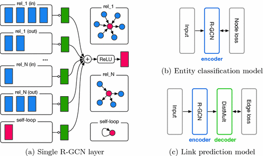
Begin by creating a learnable node-level embedding that stores a 64-element representation tensor for each node. Given that it cannot be used (negative edges are featureless) and the graph has no node features, the node embeddings here will serve as numerical features on nodes in addition to the pure structure of the graph. This embedding table is used as input to the model R-GCN, which is defined using standardized hyperparameters.
The specified model output is of width 64. Note that this number is not reflective of a number of classes: using link prediction, the R-GCN model should generate a node representation that can be used by a downstream operation to predict the probability of an edge between two nodes. There are many proposed ways to do this, including multi-layer perceptrons. This example uses the cosine similarity of the two nodes in order to generate the probability that nodes are actually connected by an edge. Thus, the model is wrapped in a link predictor module to output probabilities given input representations.
Next, define the optimizers, one for each the model itself and the embedding table. This two-optimizer setup is common within other contexts involving embedding tables, and is used to some effect here in improving model convergence.
With the components defined, it is now time to train the model. Not unlike other domains, the model can be trained on a single node using distributed data parallel (DDP) to further accelerate the model on multiple GPUs.
Once the R-GCN model has been trained, generate robust node embeddings using the network. To do this, perform graph convolution at a one-hop scale for each of the graph layers for the entire graph, and use the late-stage activations generated by the model as embeddings of the nodes of the graph.
With the node embeddings generated, join the embeddings onto the original preprocessed dataset on the respective node IDs. Next, fit an XGBoost model to the edge feature dataset augmented with the extracted embedding values from the upstream GNN model.
First, create a Dask client by connecting to the LocalCUDACluster, which is a Dask based CUDA cluster capable of executing python processes on multiple GPUs. Then the edge feature dataset is read into Dask and sampled such that the size of the final training dataset, which is defined as edge features augmented with embedding values, does not exceed 40% of the total GPU storage. This is necessary for Dask XGBoost as the full train data must be on GPU memory and the process of creating the DMatrix consumes the rest of the memory.
Next, the embeddings from the upstream model are read and the node features are appended to its corresponding ID. Finally the XGBoost model is trained to predict ‘Is Fraud?’ and it outputs the AUPRC score of 0.9 on the test set. To demonstrate the efficacy of the GNN-created node embeddings, the best XGBoost model trained on the transactions without them achieves an AUCPR score of 0.79 on the test set.
The model checkpoints can further be used to deploy this model on NVIDIA Triton Inference Server.
Once the XGBoost model has been trained, deploy the model and spin up an inference server using a Python backend to handle embedding lookup, and a Forest Inference Library (FIL) backend to perform GPU-accelerated forest library inference.
The deployment pipeline comprises three parts:
Query this service with a data sample to get the probability of the transaction being fraudulent. This probability can then be used for developing subsequent business logic.
We have performed extensive tests on one fraud detection and one benchmark dataset: TabFormer and MAG240M, respectively. To make our experiments reproducible, we have used DGX A100 (80 GB) for all the benchmark runs. This server has 64 core, dual socket AMD EPYC 7742 CPU processors and eight NVIDIA A100 (80 GB SXM4) GPU processors.
The next section presents the speedup achieved by optimizing the end-to-end workflow for GPUs.
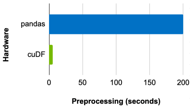
Comparing the time it takes to preprocess the dataset using pandas on a CPU and cuDF on a GPU shows a batch size of 8,192 achieves a 39x speedup with GPU (Figure 2).
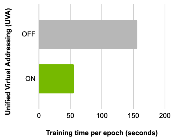
Next, comparing the training time per epoch, before and after enabling this feature, shows the advantages of using UVA. With the same batch size and a fanout of [5, 5] configuration, a 2.8x speedup is achieved on a single GPU (Figure 3).
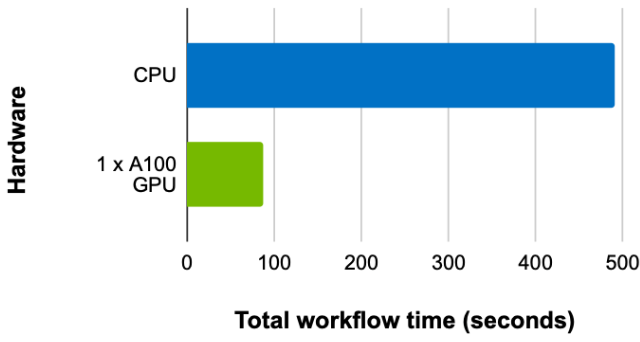
Finally, comparing the training time with the same batch size and fanout configuration, but on a CPU and a GPU (with UVA on) shows a speedup of 5.63x on a single GPU (Figure 4).
The MAG240M dataset is a part of the OGB Large Scale Challenge. It is the largest public benchmark dataset for node-level tasks with ~245 million nodes and ~1.7 billion edges.
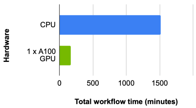
For this dataset, we first look at the total workflow time (the time it takes to preprocess the data), load, plus construct the graph and train the RGCN model. With a batch size of 4,096 and fanout of [150, 100] (used to achieve best results in hyperparameter search), we observe a ~9x speedup where the CPU takes 1,514 minutes and 1x NVIDIA A100 GPU takes 169 minutes (Figure 5).
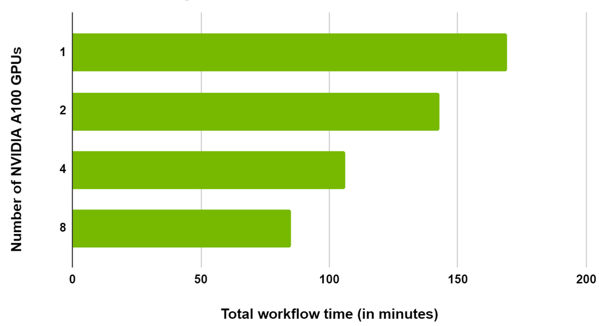
As this is a large dataset, the workflow has been scaled across multiple GPUs in the same node. We observed a 20% reduction in total time when scaling from one to two GPUs and a 50% reduction from one to eight GPUs (Figure 6).
NVIDIA has partnered with DGL and PyG to add support for graph operations on GPU and optimize preprocessing and training operations. Learn more about how NVIDIA is actively contributing to enhance these top GNN frameworks.
This post has presented an end-to-end workflow of fraud detection with GNNs including preprocessing, modeling tabular data as graph, training GNN, using GNN embeddings for downstream tasks, and deployment. This approach makes use of the NVIDIA optimized DGL, with a set of dependencies like RAPIDS cuDF and NVIDIA Triton Inference Server. We further demonstrated benchmarks on two datasets wherein we observed a 29x speedup of RGCN on MAG240M dataset on one NVIDIA A100 GPU versus CPU.
To learn more, watch the GTC session, Accelerate and Scale GNNs with Deep Graph Library and GPUs with Da Zheng, a senior applied scientist at AWS. See also Accelerating GNNs with Deep Graph Library and GPUs and Accelerating GNNs with PyTorch Geometric and GPUs, hosted by NVIDIA engineers.
If you have DGL early access or PyG early access, you can now try containers that are performance-tuned and tested for NVIDIA GPUs.