Groups across Google actively pursue research in the field of machine learning (ML), ranging from theory and application. We build ML systems to solve deep scientific and engineering challenges in areas of language, music, visual processing, algorithm development, and more. We aim to build a more collaborative ecosystem with the broader ML research community through open-sourcing tools and datasets, publishing our work, and actively participating in conferences.
Google is proud to be a Diamond Sponsor of the 40th International Conference on Machine Learning (ICML 2023), a premier annual conference, which is being held this week in Honolulu, Hawaii. As a leader in ML research, Google has a strong presence at this year’s conference with over 120 accepted papers and active involvement in a number of workshops and tutorials. Google is also proud to be a Platinum Sponsor for both the LatinX in AI and Women in Machine Learning workshops. We look forward to sharing some of our extensive ML research and expanding our partnership with the broader ML research community.
Registered for ICML 2023? We hope you’ll visit the Google booth to learn more about the exciting work, creativity, and fun that goes into solving a portion of the field’s most interesting challenges. Visit the @GoogleAI Twitter account to find out about Google booth activities (e.g., demos and Q&A sessions). See Google DeepMind’s blog to learn about their technical participation at ICML 2023.
Take a look below to learn more about the Google research being presented at ICML 2023 (Google affiliations in bold).
Board and Organizing Committee
Board Members include: Corinna Cortes, Hugo Larochelle
Tutorial Chairs include: Hanie Sedghi
Google Research booth activities
Presenters: Bryan Perozzi, Anton Tsitsulin, Brandon Mayer
Title: Unsupervised Graph Embedding @ Google (paper, EXPO workshop)
Tuesday, July 25th at 10:30 AM HST
Presenters: Zheng Xu
Title: Federated Learning of Gboard Language Models with Differential Privacy (paper 1, paper 2, blog post)
Tuesday, July 25th at 3:30 PM HST
Presenters: Thomas Kipf
Title: Self-supervised scene understanding (paper 1, paper 2)
Wednesday, July 26th at 10:30 AM HST
Presenters: Johannes von Oswald, Max Vladymyrov
Title: Transformers learn in-context by gradient descent (paper)
Wednesday, July 26th at 3:30 PM HST
Accepted papers
Scaling Vision Transformers to 22 Billion Parameters (see blog post)
Mostafa Dehghani, Josip Djolonga, Basil Mustafa, Piotr Padlewski, Jonathan Heek, Justin Gilmer, Andreas Steiner, Mathilde Caron, Robert Geirhos, Ibrahim Alabdulmohsin, Rodolphe Jenatton, Lucas Beyer, Michael Tschannen, Anurag Arnab, Xiao Wang, Carlos Riquelme, Matthias Minderer, Joan Puigcerver, Utku Evci, Manoj Kumar, Sjoerd van Steenkiste, Gamaleldin F. Elsayed, Aravindh Mahendran, Fisher Yu, Avital Oliver, Fantine Huot, Jasmijn Bastings, Mark Patrick Collier, Alexey Gritsenko, Vighnesh Birodkar, Cristina Vasconcelos, Yi Tay, Thomas Mensink, Alexander Kolesnikov, Filip Pavetić, Dustin Tran, Thomas Kipf, Mario Lučić, Xiaohua Zhai, Daniel Keysers, Jeremiah Harmsen, Neil Houlsby
Fast Inference from Transformers via Speculative Decoding
Yaniv Leviathan, Matan Kalman, Yossi Matias
Best of Both Worlds Policy Optimization
Christoph Dann, Chen-Yu Wei, Julian Zimmert
Inflow, Outflow, and Reciprocity in Machine Learning
Mukund Sundararajan, Walid Krichene
Transformers Learn In-Context by Gradient Descent
Johannes von Oswald, Eyvind Niklasson, Ettore Randazzo, João Sacramento, Alexander Mordvintsev, Andrey Zhmoginov, Max Vladymyrov
Arithmetic Sampling: Parallel Diverse Decoding for Large Language Models
Luke Vilnis, Yury Zemlyanskiy, Patrick Murray*, Alexandre Passos*, Sumit Sanghai
Differentially Private Hierarchical Clustering with Provable Approximation Guarantees (see blog post)
Jacob Imola*, Alessandro Epasto, Mohammad Mahdian, Vincent Cohen-Addad, Vahab Mirrokni
Multi-Epoch Matrix Factorization Mechanisms for Private Machine Learning
Christopher A. Choquette-Choo, H. Brendan McMahan, Keith Rush, Abhradeep Thakurta
Random Classification Noise Does Not Defeat All Convex Potential Boosters Irrespective of Model Choice
Yishay Mansour, Richard Nock, Robert Williamson
Simplex Random Features
Isaac Reid, Krzysztof Choromanski, Valerii Likhosherstov, Adrian Weller
Pix2Struct: Screenshot Parsing as Pretraining for Visual Language Understanding
Kenton Lee, Mandar Joshi, Iulia Turc, Hexiang Hu, Fangyu Liu, Julian Eisenschlos, Urvashi Khandelwal, Peter Shaw, Ming-Wei Chang, Kristina Toutanova
Mu2SLAM: Multitask, Multilingual Speech and Language Models
Yong Cheng, Yu Zhang, Melvin Johnson, Wolfgang Macherey, Ankur Bapna
Robust Budget Pacing with a Single Sample
Santiago Balseiro, Rachitesh Kumar*, Vahab Mirrokni, Balasubramanian Sivan, Di Wang
A Statistical Perspective on Retrieval-Based Models
Soumya Basu, Ankit Singh Rawat, Manzil Zaheer
Approximately Optimal Core Shapes for Tensor Decompositions
Mehrdad Ghadiri, Matthew Fahrbach, Gang Fu, Vahab Mirrokni
Efficient List-Decodable Regression Using Batches
Abhimanyu Das, Ayush Jain*, Weihao Kong, Rajat Sen
Efficient Training of Language Models Using Few-Shot Learning
Sashank J. Reddi, Sobhan Miryoosefi, Stefani Karp, Shankar Krishnan, Satyen Kale, Seungyeon Kim, Sanjiv Kumar
Fully Dynamic Submodular Maximization Over Matroids
Paul Duetting, Federico Fusco, Silvio Lattanzi, Ashkan Norouzi-Fard, Morteza Zadimoghaddam
GFlowNet-EM for Learning Compositional Latent Variable Models
Edward J Hu, Nikolay Malkin, Moksh Jain, Katie Everett, Alexandros Graikos, Yoshua Bengio
Improved Online Learning Algorithms for CTR Prediction in Ad Auctions
Zhe Feng, Christopher Liaw, Zixin Zhou
Large Language Models Struggle to Learn Long-Tail Knowledge
Nikhil Kandpal, Haikang Deng, Adam Roberts, Eric Wallace, Colin Raffel
Multi-channel Autobidding with Budget and ROI Constraints
Yuan Deng, Negin Golrezaei, Patrick Jaillet, Jason Cheuk Nam Liang, Vahab Mirrokni
Multi-layer Neural Networks as Trainable Ladders of Hilbert Spaces
Zhengdao Chen
On User-Level Private Convex Optimization
Badih Ghazi, Pritish Kamath, Ravi Kumar, Raghu Meka, Pasin Manurangsi, Chiyuan Zhang
PAC Generalization via Invariant Representations
Advait U Parulekar, Karthikeyan Shanmugam, Sanjay Shakkottai
Regularization and Variance-Weighted Regression Achieves Minimax Optimality in Linear MDPs: Theory and Practice
Toshinori Kitamura, Tadashi Kozuno, Yunhao Tang, Nino Vieillard, Michal Valko, Wenhao Yang, Jincheng Mei, Pierre Menard, Mohammad Gheshlaghi Azar, Remi Munos, Olivier Pietquin, Matthieu Geist,Csaba Szepesvari, Wataru Kumagai, Yutaka Matsuo
Speeding Up Bellman Ford via Minimum Violation Permutations
Silvio Lattanzi, Ola Svensson, Sergei Vassilvitskii
Statistical Indistinguishability of Learning Algorithms
Alkis Kalavasis, Amin Karbasi, Shay Moran, Grigoris Velegkas
Test-Time Adaptation with Slot-Centric Models
Mihir Prabhudesai, Anirudh Goyal, Sujoy Paul, Sjoerd van Steenkiste, Mehdi S. M. Sajjadi, Gaurav Aggarwal, Thomas Kipf, Deepak Pathak, Katerina Fragkiadaki>
Algorithms for Bounding Contribution for Histogram Estimation Under User-Level Privacy
Yuhan Liu*, Ananda Theertha Suresh, Wennan Zhu, Peter Kairouz, Marco Gruteser
Bandit Online Linear Optimization with Hints and Queries
Aditya Bhaskara, Ashok Cutkosky, Ravi Kumar, Manish Purohit
CLUTR: Curriculum Learning via Unsupervised Task Representation Learning
Abdus Salam Azad, Izzeddin Gur, Jasper Emhoff, Nathaniel Alexis, Aleksandra Faust, Pieter Abbeel, Ion Stoica
CSP: Self-Supervised Contrastive Spatial Pre-training for Geospatial-Visual Representations
Gengchen Mai, Ni Lao, Yutong He, Jiaming Song, Stefano Ermon
Ewald-Based Long-Range Message Passing for Molecular Graphs
Arthur Kosmala, Johannes Gasteiger, Nicholas Gao, Stephan Günnemann
Fast (1+ε)-Approximation Algorithms for Binary Matrix Factorization
Ameya Velingker, Maximilian Vötsch, David Woodruff, Samson Zhou
Federated Linear Contextual Bandits with User-Level Differential Privacy
Ruiquan Huang, Huanyu Zhang, Luca Melis, Milan Shen, Meisam Hejazinia, Jing Yang
Investigating the Role of Model-Based Learning in Exploration and Transfer
Jacob C Walker, Eszter Vértes, Yazhe Li, Gabriel Dulac-Arnold, Ankesh Anand, Theophane Weber, Jessica B Hamrick
Label Differential Privacy and Private Training Data Release
Robert Busa-Fekete, Andres Munoz, Umar Syed, Sergei Vassilvitskii
Lifelong Language Pretraining with Distribution-Specialized Experts
Wuyang Chen*, Yanqi Zhou, Nan Du, Yanping Huang, James Laudon, Zhifeng Chen, Claire Cui
Multi-User Reinforcement Learning with Low Rank Rewards
Dheeraj Mysore Nagaraj, Suhas S Kowshik, Naman Agarwal, Praneeth Netrapalli, Prateek Jain
Multi-View Masked World Models for Visual Robotic Manipulation
Younggyo Seo, Junsu Kim, Stephen James, Kimin Lee, Jinwoo Shin, Pieter Abbeel
PaLM-E: An Embodied Multimodal Language Model (see blog post)
Danny Driess, Fei Xia, Mehdi S. M. Sajjadi, Corey Lynch, Aakanksha Chowdhery, Brian Ichter,Ayzaan Wahid, Jonathan Tompson, Quan Vuong, Tianhe Yu, Wenlong Huang, Yevgen Chebotar, Pierre Sermanet, Daniel Duckworth, Sergey Levine, Vincent Vanhoucke, Karol Hausman, Marc Toussaint, Klaus Greff, Andy Zeng, Igor Mordatch, Pete Florence
Private Federated Learning with Autotuned Compression
Enayat Ullah*, Christopher A. Choquette-Choo, Peter Kairouz, Sewoong Oh
Refined Regret for Adversarial MDPs with Linear Function Approximation
Yan Dai, Haipeng Luo, Chen-Yu Wei, Julian Zimmert
Scaling Up Dataset Distillation to ImageNet-1K with Constant Memory
Justin Cui, Ruoche Wan, Si Si, Cho-Jui Hsieh
SGD with AdaGrad Stepsizes: Full Adaptivity with High Probability to Unknown Parameters, Unbounded Gradients and Affine Variance
Amit Attia, Tomer Koren
The Statistical Benefits of Quantile Temporal-Difference Learning for Value Estimation
Mark Rowland, Yunhao Tang, Clare Lyle, Rémi Munos, Marc G. Bellemare, Will Dabney
Unveiling The Mask of Position-Information Pattern Through the Mist of Image Features
Chieh Hubert Lin, Hung-Yu Tseng, Hsin-Ying Lee, Maneesh Kumar Singh, Ming-Hsuan Yang
User-Level Private Stochastic Convex Optimization with Optimal Rates
Raef Bassily, Ziteng Sun
A Simple Zero-Shot Prompt Weighting Technique to Improve Prompt Ensembling in Text-Image Models
James Urquhart Allingham*, Jie Ren, Michael W Dusenberry, Xiuye Gu, Yin Cui, Dustin Tran, Jeremiah Zhe Liu, Balaji Lakshminarayanan
Can Large Language Models Reason About Program Invariants?
Kexin Pei, David Bieber, Kensen Shi, Charles Sutton, Pengcheng Yin
Concurrent Shuffle Differential Privacy Under Continual Observation
Jay Tenenbaum, Haim Kaplan, Yishay Mansour, Uri Stemmer
Constant Matters: Fine-Grained Error Bound on Differentially Private Continual Observation
Hendrik Fichtenberger, Monika Henzinger, Jalaj Upadhyay
Cross-Entropy Loss Functions: Theoretical Analysis and Applications
Anqi Mao, Mehryar Mohri, Yutao Zhong
Efficient Rate Optimal Regret for Adversarial Contextual MDPs Using Online Function Approximation
Orin Levy, Alon Cohen, Asaf Cassel, Yishay Mansour
Fairness in Streaming Submodular Maximization Over a Matroid Constraint
Marwa El Halabi, Federico Fusco, Ashkan Norouzi-Fard, Jakab Tardos, Jakub Tarnawski
The Flan Collection: Designing Data and Methods for Effective Instruction Tuning (see blog post)
Shayne Longpre, Le Hou, Tu Vu, Albert Webson, Hyung Won Chung, Yi Tay, Denny Zhou, Quoc V Le, Barret Zoph, Jason Wei, Adam Roberts
Graph Reinforcement Learning for Network Control via Bi-level Optimization
Daniele Gammelli, James Harrison, Kaidi Yang, Marco Pavone, Filipe Rodrigues, Francisco C. Pereira
Learning-Augmented Private Algorithms for Multiple Quantile Release
Mikhail Khodak*, Kareem Amin, Travis Dick, Sergei Vassilvitskii
LegendreTron: Uprising Proper Multiclass Loss Learning
Kevin H Lam, Christian Walder, Spiridon Penev, Richard Nock
Measuring the Impact of Programming Language Distribution
Gabriel Orlanski*, Kefan Xiao, Xavier Garcia, Jeffrey Hui, Joshua Howland, Jonathan Malmaud, Jacob Austin, Rishabh Singh, Michele Catasta*
Multi-task Differential Privacy Under Distribution Skew
Walid Krichene, Prateek Jain, Shuang Song, Mukund Sundararajan, Abhradeep Thakurta, Li Zhang
Muse: Text-to-Image Generation via Masked Generative Transformers
Huiwen Chang, Han Zhang, Jarred Barber, AJ Maschinot, José Lezama, Lu Jiang, Ming-Hsuan Yang, Kevin Murphy, William T. Freeman, Michael Rubinstein, Yuanzhen Li, Dilip Krishnan
On the Convergence of Federated Averaging with Cyclic Client Participation
Yae Jee Cho, Pranay Sharma, Gauri Joshi, Zheng Xu, Satyen Kale, Tong Zhang
Optimal Stochastic Non-smooth Non-convex Optimization Through Online-to-Non-convex Conversion
Ashok Cutkosky, Harsh Mehta, Francesco Orabona
Out-of-Domain Robustness via Targeted Augmentations
Irena Gao, Shiori Sagawa, Pang Wei Koh, Tatsunori Hashimoto, Percy Liang
Polynomial Time and Private Learning of Unbounded Gaussian Mixture Models
Jamil Arbas, Hassan Ashtiani, Christopher Liaw
Pre-computed Memory or On-the-Fly Encoding? A Hybrid Approach to Retrieval Augmentation Makes the Most of Your Compute
Michiel de Jong, Yury Zemlyanskiy, Nicholas FitzGerald, Joshua Ainslie, Sumit Sanghai, Fei Sha, William W. Cohen
Scalable Adaptive Computation for Iterative Generation
Allan Jabri*, David J. Fleet, Ting Chen
Scaling Spherical CNNs
Carlos Esteves, Jean-Jacques Slotine, Ameesh Makadia
STEP: Learning N:M Structured Sparsity Masks from Scratch with Precondition
Yucheng Lu, Shivani Agrawal, Suvinay Subramanian, Oleg Rybakov, Christopher De Sa, Amir Yazdanbakhsh
Stratified Adversarial Robustness with Rejection
Jiefeng Chen, Jayaram Raghuram, Jihye Choi, Xi Wu, Yingyu Liang, Somesh Jha
When Does Privileged information Explain Away Label Noise?
Guillermo Ortiz-Jimenez*, Mark Collier, Anant Nawalgaria, Alexander D’Amour, Jesse Berent, Rodolphe Jenatton, Effrosyni Kokiopoulou
Adaptive Computation with Elastic Input Sequence
Fuzhao Xue*, Valerii Likhosherstov, Anurag Arnab, Neil Houlsby, Mostafa Dehghani, Yang You
Can Neural Network Memorization Be Localized?
Pratyush Maini, Michael C. Mozer, Hanie Sedghi, Zachary C. Lipton, J. Zico Kolter, Chiyuan Zhang
Controllability-Aware Unsupervised Skill Discovery
Seohong Park, Kimin Lee, Youngwoon Lee, Pieter Abbeel
Efficient Learning of Mesh-Based Physical Simulation with Bi-Stride Multi-Scale Graph Neural Network
Yadi Cao, Menglei Chai, Minchen Li, Chenfanfu Jiang
Federated Heavy Hitter Recovery Under Linear Sketching
Adria Gascon, Peter Kairouz, Ziteng Sun, Ananda Theertha Suresh
Graph Generative Model for Benchmarking Graph Neural Networks
Minji Yoon, Yue Wu, John Palowitch, Bryan Perozzi, Russ Salakhutdinov
H-Consistency Bounds for Pairwise Misranking Loss Surrogates
Anqi Mao, Mehryar Mohri, Yutao Zhong
Improved Regret for Efficient Online Reinforcement Learning with Linear Function Approximation
Uri Sherman, Tomer Koren, Yishay Mansour
Invariant Slot Attention: Object Discovery with Slot-Centric Reference Frames
Ondrej Biza*, Sjoerd van Steenkiste, Mehdi S. M. Sajjadi, Gamaleldin Fathy Elsayed, Aravindh Mahendran, Thomas Kipf
Multi-task Off-Policy Learning from Bandit Feedback
Joey Hong, Branislav Kveton, Manzil Zaheer, Sumeet Katariya, Mohammad Ghavamzadeh
Optimal No-Regret Learning for One-Sided Lipschitz Functions
Paul Duetting, Guru Guruganesh, Jon Schneider, Joshua Ruizhi Wang
Policy Mirror Ascent for Efficient and Independent Learning in Mean Field Games
Batuhan Yardim, Semih Cayci, Matthieu Geist, Niao He
Regret Minimization and Convergence to Equilibria in General-Sum Markov Games
Liad Erez, Tal Lancewicki, Uri Sherman, Tomer Koren, Yishay Mansour
Reinforcement Learning Can Be More Efficient with Multiple Rewards
Christoph Dann, Yishay Mansour, Mehryar Mohri
Reinforcement Learning with History-Dependent Dynamic Contexts
Guy Tennenholtz, Nadav Merlis, Lior Shani, Martin Mladenov, Craig Boutlier
User-Defined Event Sampling and Uncertainty Quantification in Diffusion Models for Physical Dynamical Systems
Marc Anton Finzi*, Anudhyan Boral, Andrew Gordon Wilson, Fei Sha, Leonardo Zepeda-Nunez
Discrete Key-Value Bottleneck
Frederik Träuble, Anirudh Goyal, Nasim Rahaman, Michael Curtis Mozer, Kenji Kawaguchi, Yoshua Bengio, Bernhard Schölkopf
DSGD-CECA: Decentralized SGD with Communication-Optimal Exact Consensus Algorithm
Lisang Ding, Kexin Jin, Bicheng Ying, Kun Yuan, Wotao Yin
Exphormer: Sparse Transformers for Graphs
Hamed Shirzad, Ameya Velingker, Balaji Venkatachalam, Danica J. Sutherland, Ali Kemal Sinop
Fast, Differentiable and Sparse Top-k: A Convex Analysis Perspective
Michael Eli Sander*, Joan Puigcerver, Josip Djolonga, Gabriel Peyré, Mathieu Blondel
Improved Policy Evaluation for Randomized Trials of Algorithmic Resource Allocation
Aditya Mate, Bryan Wilder, Aparna Taneja, Milind Tambe
In Search for a Generalizable Method for Source Free Domain Adaptation
Malik Boudiaf*, Tom Denton, Bart van Merrienboer, Vincent Dumoulin, Eleni Triantafillou
Learning Rate Schedules in the Presence of Distribution Shift
Matthew Fahrbach, Adel Javanmard, Vahab Mirrokni, Pratik Worah
Not All Semantics Are Created Equal: Contrastive Self-Supervised Learning with Automatic Temperature Individualization
Zi-Hao Qiu, Quanqi Hu, Zhuoning Yuan, Denny Zhou, Lijun Zhang, Tianbao Yang
On the Relationship Between Explanation and Prediction: A Causal View
Amir-Hossein Karimi*, Krikamol Muandet, Simon Kornblith, Bernhard Schölkopf, Been Kim
On the Role of Attention in Prompt-Tuning
Samet Oymak, Ankit Singh Rawat, Mahdi Soltanolkotabi, Christos Thrampoulidis
PLay: Parametrically Conditioned Layout Generation Using Latent Diffusion
Chin-Yi Cheng, Forrest Huang, Gang Li, Yang Li
The Power of Learned Locally Linear Models for Nonlinear Policy Optimization
Daniel Pfrommer, Max Simchowitz, Tyler Westenbroek, Nikolai Matni, Stephen Tu
Relevant Walk Search for Explaining Graph Neural Networks
Ping Xiong, Thomas Schnake, Michael Gastegger, Grégoire Montavon, Klaus Robert Muller,Shinichi Nakajima
Repository-Level Prompt Generation for Large Language Models of Code
Disha Shrivastava, Hugo Larochelle, Daniel Tarlow
Robust and Private Stochastic Linear Bandits
Vasileios Charisopoulos*, Hossein Esfandiari, Vahab Mirrokni
Simple Diffusion: End-to-End Diffusion for High Resolution Images
Emiel Hoogeboom, Jonathan Heek, Tim Salimans
Tied-Augment: Controlling Representation Similarity Improves Data Augmentation
Emirhan Kurtulus, Zichao Li, Yann Dauphin, Ekin D. Cubuk
Why Is Public Pre-Training Necessary for Private Model Training?
Arun Ganesh, Mahdi Haghifam*, Milad Nasr, Sewoong Oh, Thomas Steinke, Om Thakkar, Abhradeep Guha Thakurta, Lun Wang
A Connection Between One-Step RL and Critic Regularization in Reinforcement Learning
Benjamin Eysenbach, Matthieu Geist, Sergey Levine, Ruslan Salakhutdinov
Beyond Uniform Lipschitz Condition in Differentially Private Optimization
Rudrajit Das*, Satyen Kale, Zheng Xu, Tong Zhang, Sujay Sanghavi
Efficient Graph Field Integrators Meet Point Clouds
Krzysztof Choromanski, Arijit Sehanobish, Han Lin, Yunfan Zhao, Eli Berger, Tetiana Parshakova, Alvin Pan, David Watkins, Tianyi Zhang, Valerii Likhosherstov, Somnath Basu Roy Chowdhury, Avinava Dubey, Deepali Jain, Tamas Sarlos, Snigdha Chaturvedi, Adrian Weller
Fast as CHITA: Neural Network Pruning with Combinatorial Optimization
Riade Benbaki, Wenyu Chen, Xiang Meng, Hussein Hazimeh, Natalia Ponomareva, Zhe Zhao, Rahul Mazumder
Jump-Start Reinforcement Learning (see blog post)
Ikechukwu Uchendu*, Ted Xiao, Yao Lu, Banghua Zhu, Mengyuan Yan, Joséphine Simon, Matthew Bennice, Chuyuan Fu, Cong Ma, Jiantao Jiao, Sergey Levine, Karol Hausman
Learning in POMDPs is Sample-Efficient with Hindsight Observability
Jonathan Lee, Alekh Agarwal, Christoph Dann, Tong Zhang
Low-Variance Gradient Estimation in Unrolled Computation Graphs with ES-Single
Paul Vicol
Masked Trajectory Models for Prediction, Representation, and Control
Philipp Wu, Arjun Majumdar, Kevin Stone, Yixin Lin, Igor Mordatch, Pieter Abbeel, Aravind Rajeswaran
Overcoming Simplicity Bias in Deep Networks Using a Feature Sieve
Rishabh Tiwari, Pradeep Shenoy
Pairwise Ranking Losses of Click-Through Rates Prediction for Welfare Maximization in Ad Auctions
Boxiang Lyu, Zhe Feng, Zachary Robertson, Sanmi Koyejo
Predictive Flows for Faster Ford-Fulkerson
Sami Davies, Benjamin Moseley, Sergei Vassilvitskii, Yuyan Wang
Scaling Laws for Multilingual Neural Machine Translation
Patrick Fernandes, Behrooz Ghorbani, Xavier Garcia, Markus Freitag, Orhan Firat
Sequential Monte Carlo Learning for Time Series Structure Discovery
Feras Saad, Brian Patton, Matthew Douglas Hoffman, Rif A. Saurous, Vikash Mansinghka
Stochastic Gradient Succeeds for Bandits
Jincheng Mei, Zixin Zhong, Bo Dai, Alekh Agarwal, Csaba Szepesvari, Dale Schuurmans
Subset-Based Instance Optimality in Private Estimation
Travis Dick, Alex Kulesza, Ziteng Sun, Ananda Theertha Suresh
The Unreasonable Effectiveness of Few-Shot Learning for Machine Translation
Xavier Garcia, Yamini Bansal, Colin Cherry, George Foster, Maxim Krikun, Melvin Johnson, Orhan Firat
Tutorials
Self-Supervised Learning in Vision: from Research Advances to Best Practices
Xinlei Chen, Ishan Misra, Randall Balestriero, Mathilde Caron, Christoph Feichtenhofer, Mark Ibrahim
How to DP-fy ML: A Practical Tutorial to Machine Learning with Differential Privacy (see blog post)
Sergei Vassilvitskii, Natalia Ponomareva, Zheng Xu
Recent Advances in the Generalization Theory of Neural Networks
Tengyu Ma, Alex Damian
EXPO Day workshops
Graph Neural Networks in Tensorflow: A Practical Guide
Workshop Organizers include: Bryan Perozzi, Anton Tsitsulin, Brandon Mayer, Jonathan Halcrow
Google sponsored affinity workshops
LatinX in AI (LAXAI)
Platinum Sponsor
Keynote Speaker: Monica Ribero
Panelist: Yao Qin
Women in Machine Learning (WiML)
Platinum Sponsor
Panelists: Yao Qin
Workshops
Federated Learning and Analytics in Practice: Algorithms, Systems, Applications, and Opportunities
Organizer: Peter Kairouz, Zheng Xu
Speaker: Brendan McMahan
Interpretable Machine Learning in Healthcare (IMLH)
Organizer: Ramin Zabih
Knowledge and Logical Reasoning in the Era of Data-Driven Learning
Organizer: Beliz Günel
The Many Facets of Preference-Based Learning (MFPL)
Organizer: Robert Busa-Fekete, Mohammad Ghavamzadeh
The Synergy of Scientific and Machine Learning Modelling (SynS & ML)
Speaker: Sercan Arik
Theory of Mind in Communicating Agents
Organizer: Pei Zhou
Artificial Intelligence & Human Computer Interaction
Organizer: Yang Li, Forrest Huang
Data-Centric Machine Learning Research (DMLR)
Organizer: Alicia Parrish, Najoung Kim
Speaker: Peter Mattson
Neural Compression: from Information Theory to Applications
Speaker: Johannes Ballé
Panelist: George Toderici
Organizer: Ahmad Beirami
Spurious Correlations, Invariance and Stability (SCIS)
Organizer: Amir Feder
* Work done while at Google


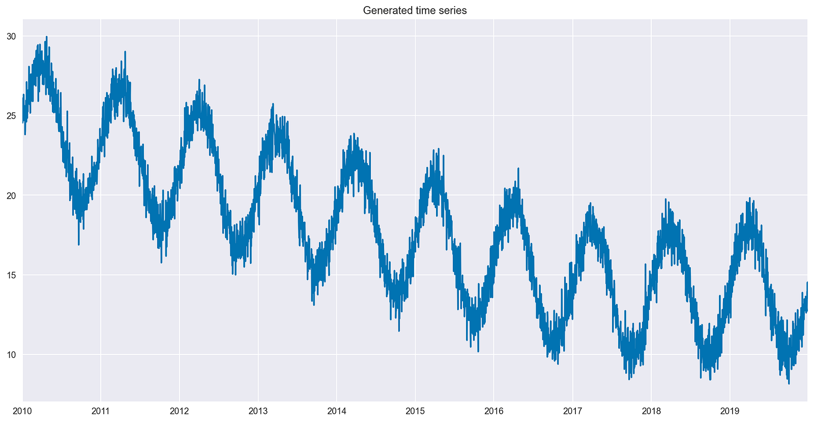
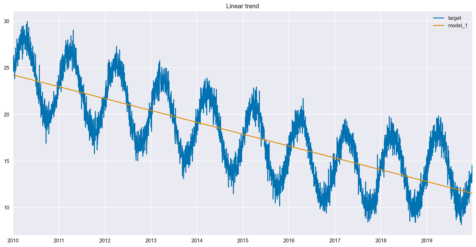
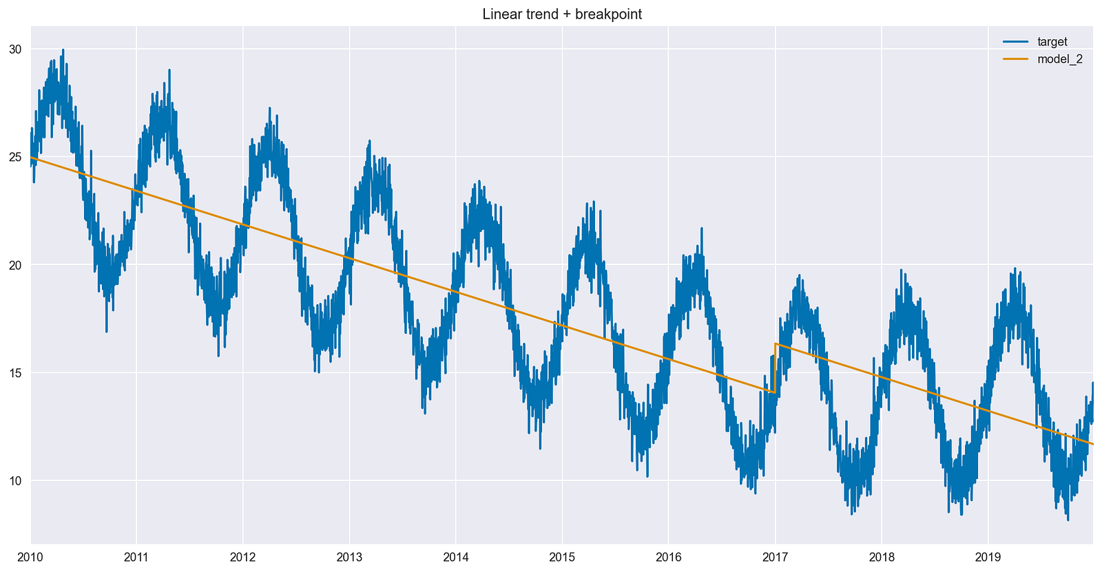
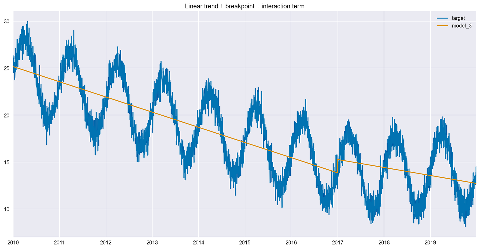
 Modeling time series data can be challenging (and fascinating) due to its inherent complexity and unpredictability. Long-term trends in time series can change…
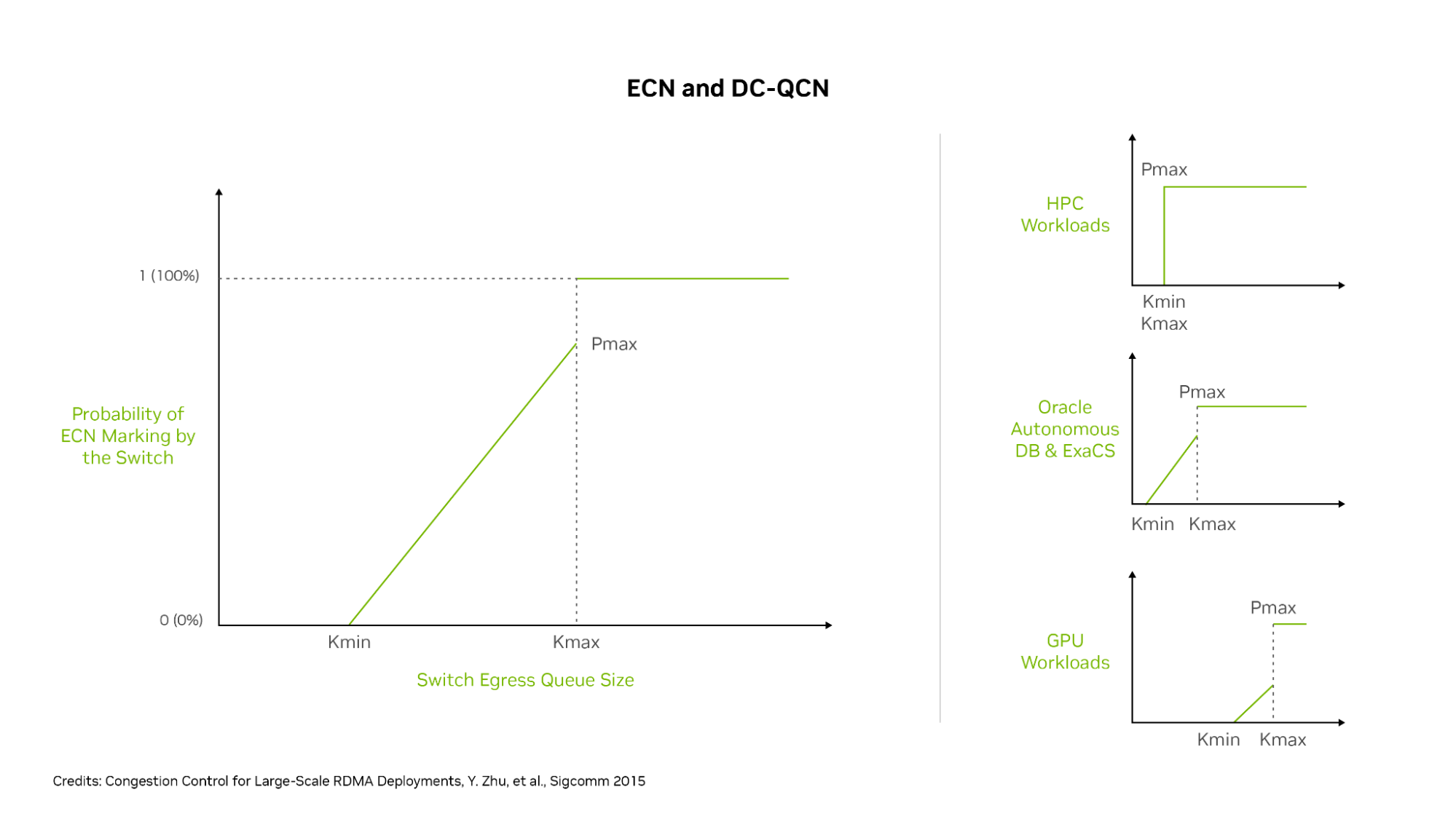
 Oracle is one of the top cloud service providers in the world, supporting over 22,000 customers and reporting revenue of nearly $4 billion per quarter and…
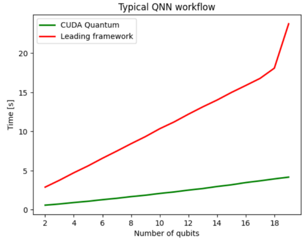
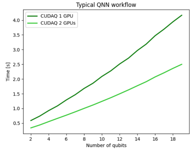
 Heterogeneous computing architectures—those that incorporate a variety of processor types working in tandem—have proven extremely valuable in the continued…
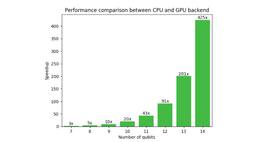


 Pipeline state objects (PSOs) define how input data is interpreted and rendered by the hardware when submitting work to the GPUs. Proper management of PSOs is…
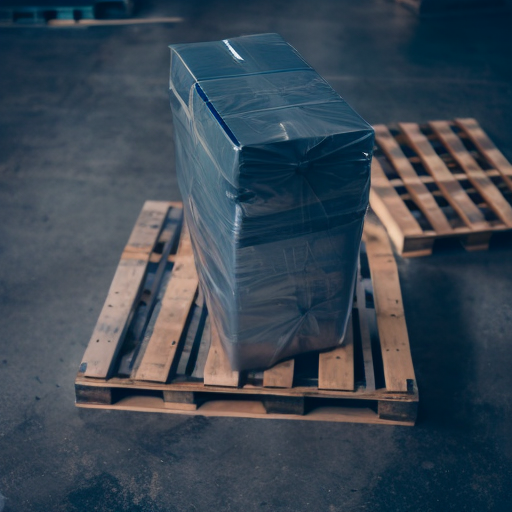
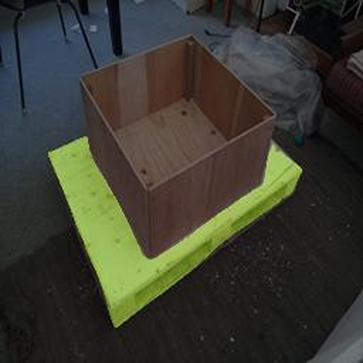
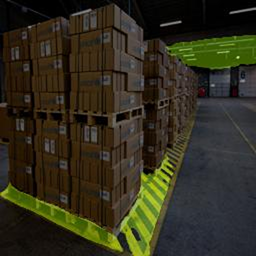
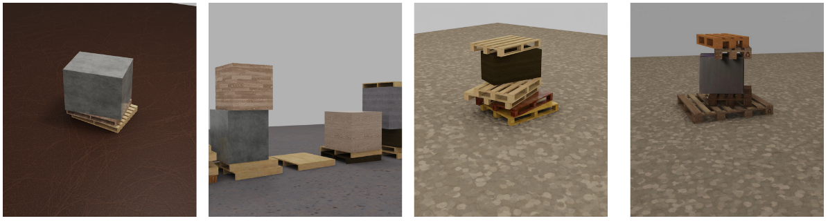
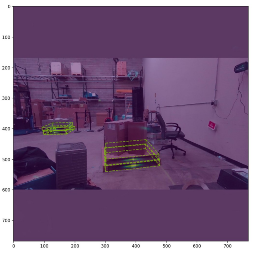
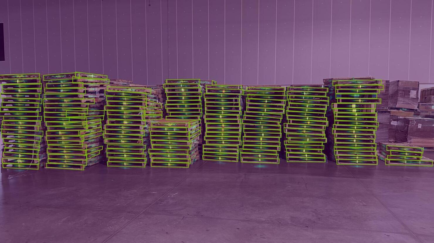
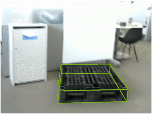
 Imagine you are a robotics or machine learning (ML) engineer tasked with developing a model to detect pallets so that a forklift can manipulate them. You are…
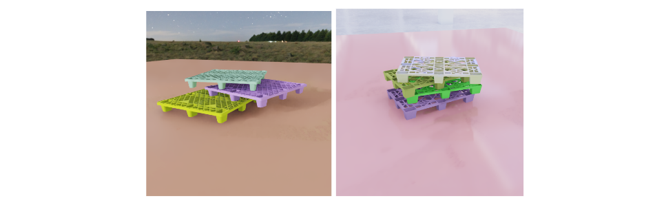
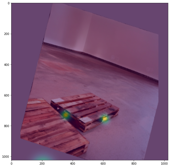
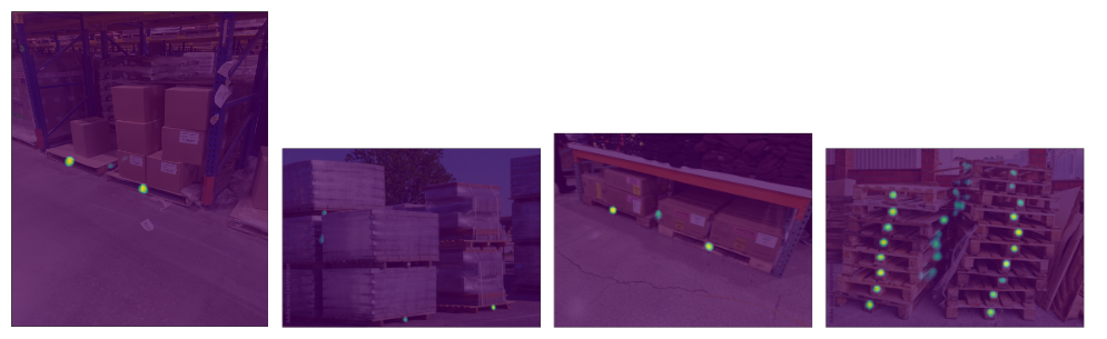
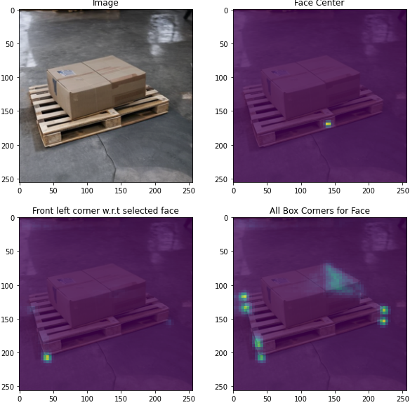