 Graph neural networks (GNNs) have emerged as a powerful tool for a variety of machine learning tasks on graph-structured data. These tasks range from node…
Graph neural networks (GNNs) have emerged as a powerful tool for a variety of machine learning tasks on graph-structured data. These tasks range from node classification and link prediction to graph classification. They also cover a wide range of applications such as social network analysis, drug discovery in healthcare, fraud detection in financial services, and molecular chemistry.
In this post, I introduce how to use cuGraph-DGL, a GPU-accelerated library for graph computations. It extends Deep Graph Library (DGL), a popular framework for GNNs that enables large-scale applications.
Basics of graph neural networks
Before I dive into cuGraph-DGL, I want to establish some basics. GNNs are a special kind of neural network designed to work with data structured as graphs. Unlike traditional neural networks that assume independence between samples, which doesn’t fit well with graph data, GNNs effectively exploit the rich and complex interconnections within graph data.
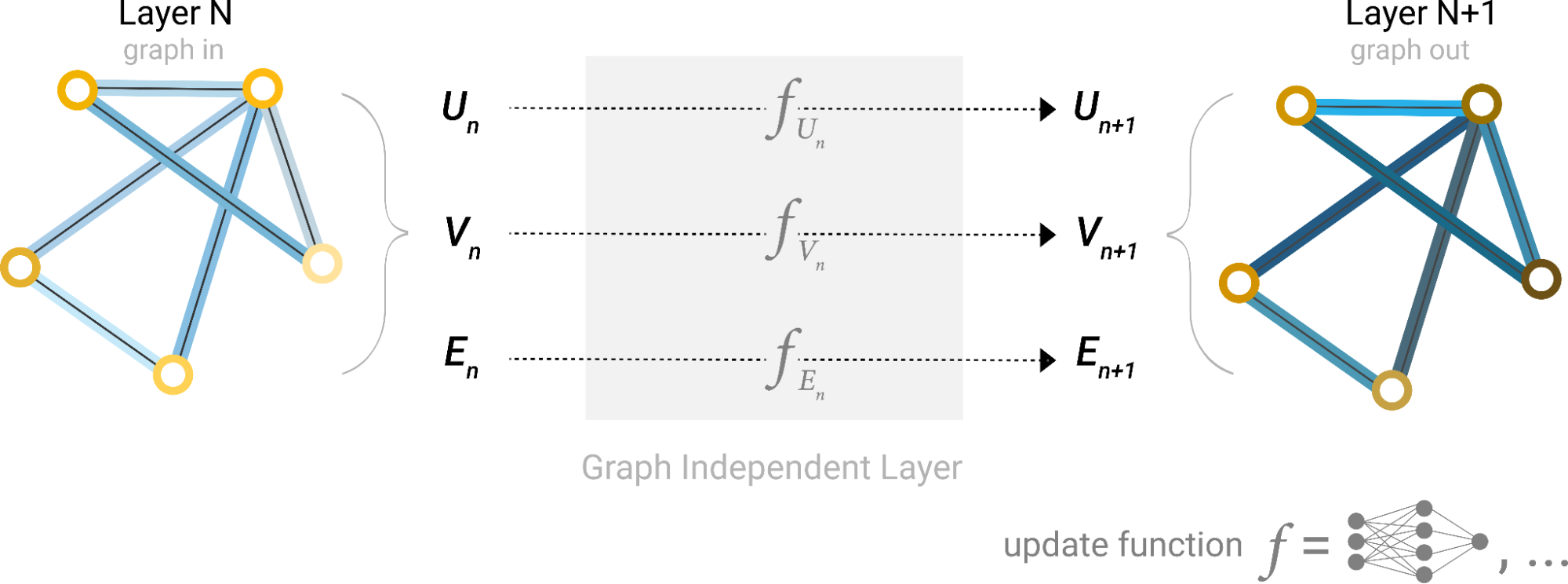
In a nutshell, GNNs work by propagating and transforming node features across the graph structure in multiple steps, often referred to as layers (Figure 1). Each layer updates the features of each node based on its own features and the features of its neighbors.

In Figure 1, the first step “prepares” a message composed of information from an edge and its connected nodes and then “passes” the message to the node. This process enables the model to learn high-level representations of nodes, edges, and the graph as a whole, which can be used for various downstream tasks like node classification, link prediction, and graph classification.
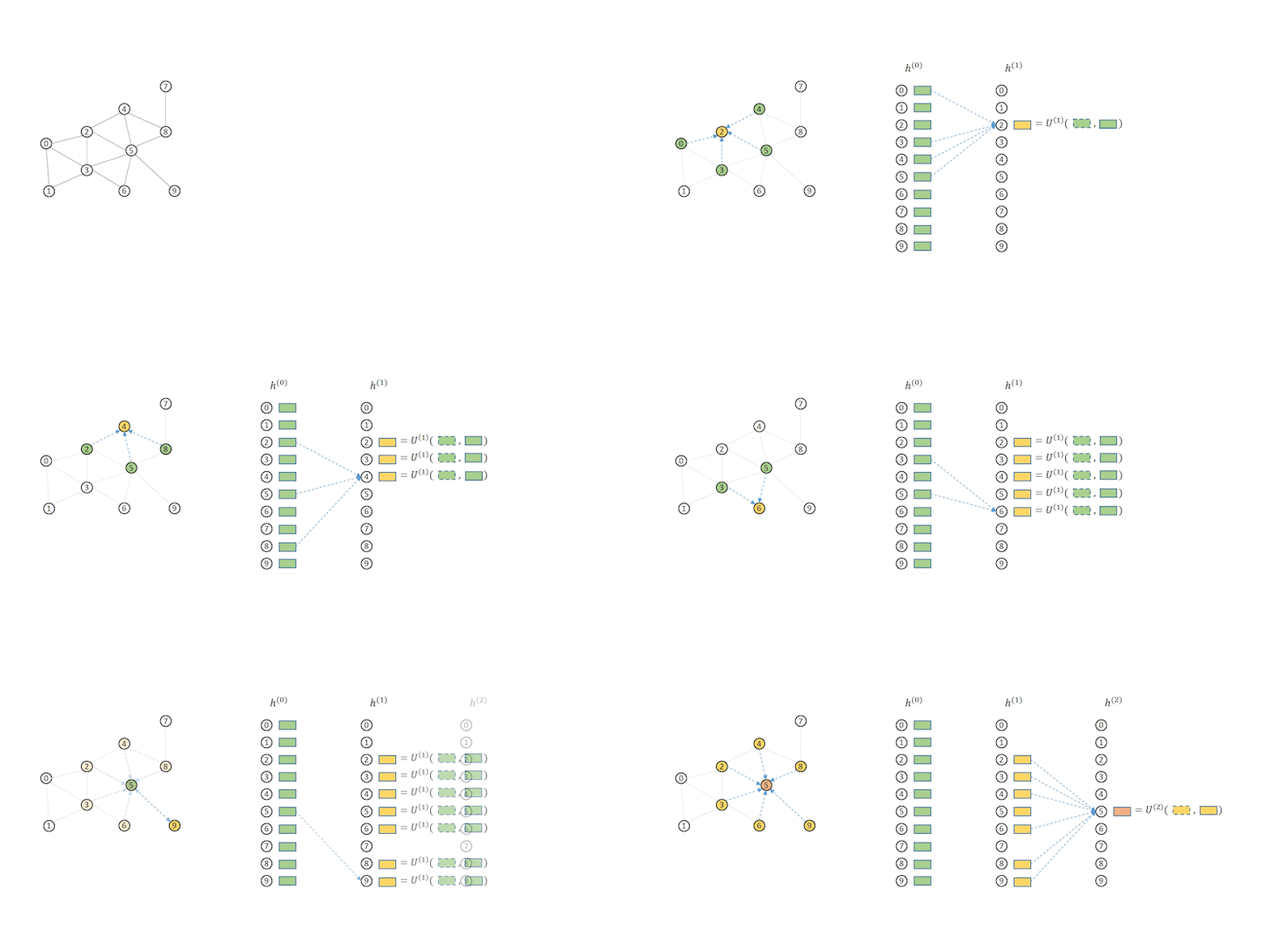
Figure 2 shows how a 2-layer GNN is supposed to compute the output of node 5.

Bottlenecks when handling large-scale graphs
The bottleneck in GNN sampling and training is the lack of an existing implementation that can scale to handle billions or even trillions of edges, a scale often seen in real-world graph problems. For example, if you’re handling a graph with trillions of edges, you must be able to run DGL-based GNN workflows quickly.
One solution is to use RAPIDS, which already possesses the foundational elements capable of scaling to trillions of edges using GPUs.
What is RAPIDS cuGraph?
cuGraph is a part of the RAPIDS AI ecosystem, an open-source suite of software libraries for executing end-to-end data science and analytics pipelines entirely on GPUs. The cuGraph library provides a simple, flexible, and powerful API for graph analytics, enabling you to perform computations on graph data at scale and speed.
What is DGL?
Deep Graph Library (DGL) is a Python library designed to simplify the implementation of graph neural networks (GNNs) by providing intuitive interfaces and high-performance computation.
DGL supports a broad array of graph operations and structures, enhancing the modeling of complex systems and relationships. It also integrates with popular deep learning frameworks like PyTorch and TensorFlow, fostering seamless development and deployment of GNNs.
What is cuGraph-DGL?
cuGraph-DGL is an extension of cuGraph that integrates with the Deep Graph Library (DGL) to leverage the power of GPUs to run DGL-based GNN workflows at unprecedented speed. This library is a collaborative effort between DGL developers and cuGraph developers.
In addition to cuGraph-DGL, cuGraph also provides the cugraph-ops library, which enables DGL users to get performance boosts using CuGraphSAGEConv, CuGraphGATConv, and CuGraphRelGraphConv in place of the default SAGEConv, GATConv, and RelGraphConv models. You can also import the SAGEConv, GATConv, and RelGraphConv models directly from the cugraph_dgl library.
In GNN sampling and training, the major challenge is the absence of an implementation that can manage real-world graph problems with billions or trillions of edges. To address this, use cuGraph-DGL, with its inherent capability to scale to trillions of edges using GPUs.
Setting up cuGraph-DGL
Before you dive into the code, make sure that you have cuGraph and DGL installed in your Python environment. To install the cuGraph-DGL-enabled environment, run the following command:
conda install mamba -c conda-forge

mamba create -n cugraph_dgl_23_06 -c pytorch -c dglteam/label/cu118 -c rapidsai-nightly -c nvidia -c conda-forge dgl cugraph-dgl=23.10 pylibcugraphops=23.10 cudatoolkit=11.8 torchmetrics ogb
Implementing a GNN with cuGraph-DGL
With your environment set up, put cuGraph-DGL into action and construct a simple GNN for node classification. Converting an existing DGL workflow to a cuGraph-DGL workflow has the following steps:
- Use cuGraph-ops models such as
CuGraphSAGECon, in place of the native DGL model (SAGEConv). - Create a
CuGraphGraphobject from a DGL graph. - Use the
cuGraphdata loader in place of the native DGL Dataloader.
Using cugraph-dgl on a 3.2 billion-edge graph, we observed a 3x speedup when using eight GPUs for sampling and training, compared to a single GPU UVA DGL setup. Additionally, we saw a 2x speedup when using eight GPUs for sampling and one GPU for training.
An upcoming blog post will provide more details on the gains and scalability.
Create a cuGraph-DGL graph
To create a cugraph_dgl graph directly from a DGL graph, run the following code example.
import dgl
import cugraph_dgl

dataset = dgl.data.CoraGraphDataset()
dgl_g = dataset[0]
# Add self loops as cugraph
# does not support isolated vertices yet
dgl_g = dgl.add_self_loop(dgl_g)
cugraph_g = cugraph_dgl.convert.cugraph_storage_from_heterograph(dgl_g, single_gpu=True)
For more information about creating a cuGraph storage object, see CuGraphStorage.
Create a cuGraph-Ops-based model
In this step, the only modification to make is the importation of cugraph_ops-based models. These models are drop-in replacements for upstream models like dgl.nn.SAGECon.
# Drop in replacement for dgl.nn.SAGEConv
from dgl.nn import CuGraphSAGEConv as SAGEConv

import torch.nn as nn
import torch.nn.functional as F

class SAGE(nn.Module):
    def __init__(self, in_size, hid_size, out_size):
        super().__init__()
        self.layers = nn.ModuleList()
        # three-layer GraphSAGE-mean
        self.layers.append(SAGEConv(in_size, hid_size, "mean"))
        self.layers.append(SAGEConv(hid_size, hid_size, "mean"))
        self.layers.append(SAGEConv(hid_size, out_size, "mean"))
        self.dropout = nn.Dropout(0.5)
        self.hid_size = hid_size
        self.out_size = out_size

    def forward(self, blocks, x):
        h = x
        for l_id, (layer, block) in enumerate(zip(self.layers, blocks)):
            h = layer(block, h)
            if l_id != len(self.layers) - 1:
                h = F.relu(h)
                h = self.dropout(h)
        return h


# Create the model with given dimensions
feat_size = cugraph_g.ndata["feat"]["_N"].shape[1]
model = SAGE(feat_size, 256, dataset.num_classes).to("cuda")
Train the model
In this step, you opt to use cugraph_dgl.dataloading.NeighborSampler and cugraph_dgl.dataloading.DataLoader, replacing the conventional data loaders of upstream DGL.
import torchmetrics.functional as MF
import tempfile
import torch

def train(g, model):
    optimizer = torch.optim.Adam(model.parameters(), lr=0.01)

    features = g.ndata["feat"]["_N"].to("cuda")
    labels = g.ndata["label"]["_N"].to("cuda")
    train_nid = torch.tensor(range(g.num_nodes())).type(torch.int64)
    temp_dir_name = tempfile.TemporaryDirectory().name

    for epoch in range(10):
        model.train()
        sampler = cugraph_dgl.dataloading.NeighborSampler([10,10,10])
        dataloader = cugraph_dgl.dataloading.DataLoader(g, train_nid, sampler,
                                                batch_size=128,
                                                shuffle=True,
                                                drop_last=False,
                                                num_workers=0,
                                                sampling_output_dir=temp_dir_name)

        total_loss = 0

        for step, (input_nodes, seeds, blocks) in enumerate((dataloader)):
            batch_inputs = features[input_nodes]
            batch_labels = labels[seeds]
            batch_pred = model(blocks, batch_inputs)
            loss = F.cross_entropy(batch_pred, batch_labels)
            total_loss += loss
            optimizer.zero_grad()
            loss.backward()
            optimizer.step()


        sampler = cugraph_dgl.dataloading.NeighborSampler([-1,-1,-1])
        dataloader = cugraph_dgl.dataloading.DataLoader(g, train_nid, sampler,
                                                batch_size=1024,
                                                shuffle=False,
                                                drop_last=False,
                                                num_workers=0,
                                                sampling_output_dir=temp_dir_name)


        acc = evaluate(model, features, labels, dataloader)
        print("Epoch {:05d} | Acc {:.4f} | Loss {:.4f} ".format(epoch, acc, total_loss))


def evaluate(model, features, labels, dataloader):
    with torch.no_grad():
        model.eval()
        ys = []
        y_hats = []
        for it, (in_nodes, out_nodes, blocks) in enumerate(dataloader):
            with torch.no_grad():
                x = features[in_nodes]
                ys.append(labels[out_nodes])
                y_hats.append(model(blocks, x))
        num_classes = y_hats[0].shape[1]
        return MF.accuracy(
            torch.cat(y_hats),
            torch.cat(ys),
            task="multiclass",
            num_classes=num_classes,
        )

train(cugraph_g, model)

Epoch 00000 | Acc 0.3401 | Loss 39.3890
Epoch 00001 | Acc 0.7164 | Loss 27.8906
Epoch 00002 | Acc 0.7888 | Loss 16.9441
Epoch 00003 | Acc 0.8589 | Loss 12.5475
Epoch 00004 | Acc 0.8863 | Loss 9.9894
Epoch 00005 | Acc 0.8948 | Loss 9.0556
Epoch 00006 | Acc 0.9029 | Loss 7.3637
Epoch 00007 | Acc 0.9055 | Loss 7.2541
Epoch 00008 | Acc 0.9132 | Loss 6.6912
Epoch 00009 | Acc 0.9121 | Loss 7.0908
Conclusion
By combining the power of GPU-accelerated graph computations with the flexibility of DGL, cuGraph-DGL emerges as an invaluable tool for anyone dealing with graph data.
This post has only scratched the surface of what you can do with cuGraph-DGL. I encourage you to explore further, experiment with different GNN architectures, and discover how cuGraph-DGL can accelerate your graph-based, machine-learning tasks.
Read Intro to Graph Neural Networks with cuGraph-PyG for details on how to implement GNNs in the cuGraph-PyG ecosystem
