Routing in Google Maps remains one of our most helpful and frequently used features. Determining the best route from A to B requires making complex trade-offs between factors including the estimated time of arrival (ETA), tolls, directness, surface conditions (e.g., paved, unpaved roads), and user preferences, which vary across transportation mode and local geography. Often, the most natural visibility we have into travelers’ preferences is by analyzing real-world travel patterns.
Learning preferences from observed sequential decision making behavior is a classic application of inverse reinforcement learning (IRL). Given a Markov decision process (MDP) — a formalization of the road network — and a set of demonstration trajectories (the traveled routes), the goal of IRL is to recover the users’ latent reward function. Although past research has created increasingly general IRL solutions, these have not been successfully scaled to world-sized MDPs. Scaling IRL algorithms is challenging because they typically require solving an RL subroutine at every update step. At first glance, even attempting to fit a world-scale MDP into memory to compute a single gradient step appears infeasible due to the large number of road segments and limited high bandwidth memory. When applying IRL to routing, one needs to consider all reasonable routes between each demonstration’s origin and destination. This implies that any attempt to break the world-scale MDP into smaller components cannot consider components smaller than a metropolitan area.
To this end, in “Massively Scalable Inverse Reinforcement Learning in Google Maps“, we share the result of a multi-year collaboration among Google Research, Maps, and Google DeepMind to surpass this IRL scalability limitation. We revisit classic algorithms in this space, and introduce advances in graph compression and parallelization, along with a new IRL algorithm called Receding Horizon Inverse Planning (RHIP) that provides fine-grained control over performance trade-offs. The final RHIP policy achieves a 16–24% relative improvement in global route match rate, i.e., the percentage of de-identified traveled routes that exactly match the suggested route in Google Maps. To the best of our knowledge, this represents the largest instance of IRL in a real world setting to date.
 |
| Google Maps improvements in route match rate relative to the existing baseline, when using the RHIP inverse reinforcement learning policy. |
The benefits of IRL
A subtle but crucial detail about the routing problem is that it is goal conditioned, meaning that every destination state induces a slightly different MDP (specifically, the destination is a terminal, zero-reward state). IRL approaches are well suited for these types of problems because the learned reward function transfers across MDPs, and only the destination state is modified. This is in contrast to approaches that directly learn a policy, which typically require an extra factor of S parameters, where S is the number of MDP states.
Once the reward function is learned via IRL, we take advantage of a powerful inference-time trick. First, we evaluate the entire graph’s rewards once in an offline batch setting. This computation is performed entirely on servers without access to individual trips, and operates only over batches of road segments in the graph. Then, we save the results to an in-memory database and use a fast online graph search algorithm to find the highest reward path for routing requests between any origin and destination. This circumvents the need to perform online inference of a deeply parameterized model or policy, and vastly improves serving costs and latency.
 |
| Reward model deployment using batch inference and fast online planners. |
Receding Horizon Inverse Planning
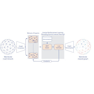
To scale IRL to the world MDP, we compress the graph and shard the global MDP using a sparse Mixture of Experts (MoE) based on geographic regions. We then apply classic IRL algorithms to solve the local MDPs, estimate the loss, and send gradients back to the MoE. The worldwide reward graph is computed by decompressing the final MoE reward model. To provide more control over performance characteristics, we introduce a new generalized IRL algorithm called Receding Horizon Inverse Planning (RHIP).
 |
| IRL reward model training using MoE parallelization, graph compression, and RHIP. |
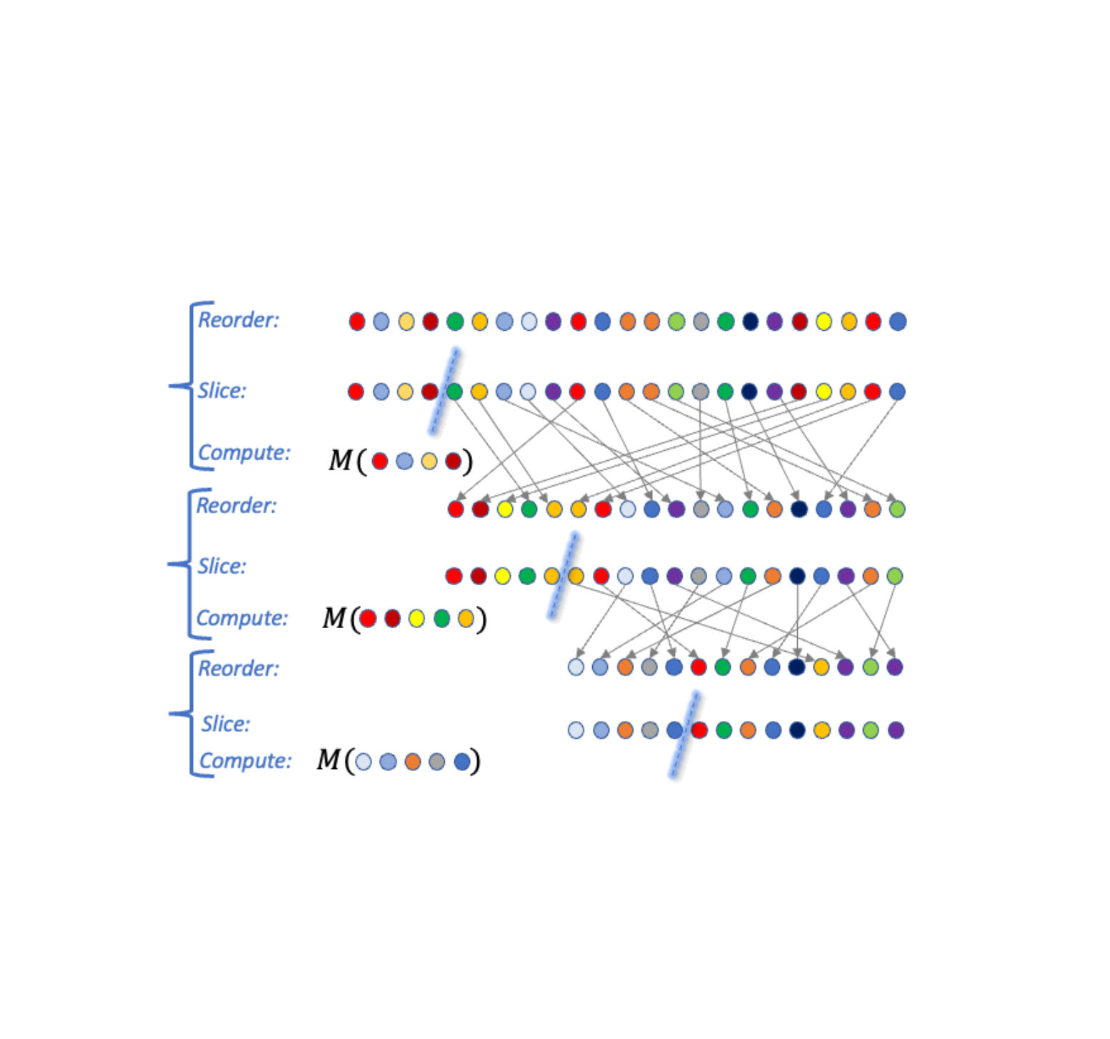
RHIP is inspired by people’s tendency to perform extensive local planning (“What am I doing for the next hour?”) and approximate long-term planning (“What will my life look like in 5 years?”). To take advantage of this insight, RHIP uses robust yet expensive stochastic policies in the local region surrounding the demonstration path, and switches to cheaper deterministic planners beyond some horizon. Adjusting the horizon H allows controlling computational costs, and often allows the discovery of the performance sweet spot. Interestingly, RHIP generalizes many classic IRL algorithms and provides the novel insight that they can be viewed along a stochastic vs. deterministic spectrum (specifically, for H=∞ it reduces to MaxEnt, for H=1 it reduces to BIRL, and for H=0 it reduces to MMP).
 |
| Given a demonstration from so to sd, (1) RHIP follows a robust yet expensive stochastic policy in the local region surrounding the demonstration (blue region). (2) Beyond some horizon H, RHIP switches to following a cheaper deterministic planner (red lines). Adjusting the horizon enables fine-grained control over performance and computational costs. |
Routing wins
The RHIP policy provides a 15.9% and 24.1% lift in global route match rate for driving and two-wheelers (e.g., scooters, motorcycles, mopeds) relative to the well-tuned Maps baseline, respectively. We’re especially excited about the benefits to more sustainable transportation modes, where factors beyond journey time play a substantial role. By tuning RHIP’s horizon H, we’re able to achieve a policy that is both more accurate than all other IRL policies and 70% faster than MaxEnt.
Our 360M parameter reward model provides intuitive wins for Google Maps users in live A/B experiments. Examining road segments with a large absolute difference between the learned rewards and the baseline rewards can help improve certain Google Maps routes. For example:
 |
| Nottingham, UK. The preferred route (blue) was previously marked as private property due to the presence of a large gate, which indicated to our systems that the road may be closed at times and would not be ideal for drivers. As a result, Google Maps routed drivers through a longer, alternate detour instead (red). However, because real-world driving patterns showed that users regularly take the preferred route without an issue (as the gate is almost never closed), IRL now learns to route drivers along the preferred route by placing a large positive reward on this road segment. |
Conclusion
Increasing performance via increased scale – both in terms of dataset size and model complexity – has proven to be a persistent trend in machine learning. Similar gains for inverse reinforcement learning problems have historically remained elusive, largely due to the challenges with handling practically sized MDPs. By introducing scalability advancements to classic IRL algorithms, we’re now able to train reward models on problems with hundreds of millions of states, demonstration trajectories, and model parameters, respectively. To the best of our knowledge, this is the largest instance of IRL in a real-world setting to date. See the paper to learn more about this work.
Acknowledgements
This work is a collaboration across multiple teams at Google. Contributors to the project include Matthew Abueg, Oliver Lange, Matt Deeds, Jason Trader, Denali Molitor, Markus Wulfmeier, Shawn O’Banion, Ryan Epp, Renaud Hartert, Rui Song, Thomas Sharp, Rémi Robert, Zoltan Szego, Beth Luan, Brit Larabee and Agnieszka Madurska.
We’d also like to extend our thanks to Arno Eigenwillig, Jacob Moorman, Jonathan Spencer, Remi Munos, Michael Bloesch and Arun Ahuja for valuable discussions and suggestions.
 Spear phishing is the largest and most costly form of cyber threat, with an estimated 300,000 reported victims in 2021 representing $44 million in reported…
 On Sept. 27, join us to learn recommender systems best practices for building, training, and deploying at any scale.
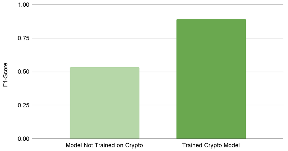
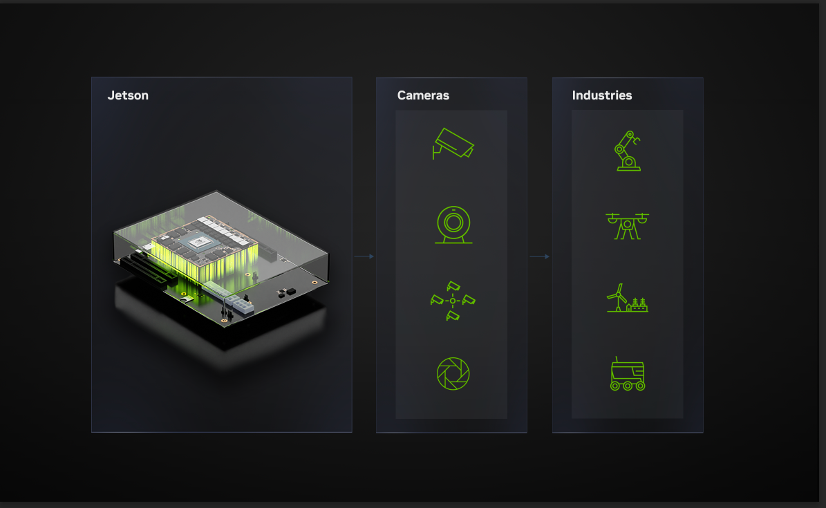
 The camera module is the most integral part of an AI-based embedded system. With so many camera module choices on the market, the selection process may seem…


 Explore how ray-traced caustics combined with NVIDIA RTX features can enhance the performance of your games.