Video is a core data path across NVIDIA Jetson applications, from robotics and intelligent video analytics to industrial automation, healthcare, media…
Video is a core data path across NVIDIA Jetson applications, from robotics and intelligent video analytics to industrial automation, healthcare, media processing, and remote operations. A system may capture several cameras, decode network streams, run AI inference or conventional vision processing, draw results, and encode video for storage or delivery. The individual calls are…
AI infrastructure spans multiple layers, from compute and networking to storage, orchestration, and applications. When performance degrades, identifying the…
AI infrastructure spans multiple layers, from compute and networking to storage, orchestration, and applications. When performance degrades, identifying the source can be difficult because a symptom observed at one layer may originate elsewhere in the stack. A full-stack observability strategy connects telemetry across these layers, helping infrastructure and operations teams detect problems…
Alibaba released the open weights for Qwen3.8-2.4T-A95B (Qwen3.8-Max), its largest open-weight model, bringing near-frontier capabilities to the open…
Alibaba released the open weights for Qwen3.8-2.4T-A95B (Qwen3.8-Max), its largest open-weight model, bringing near-frontier capabilities to the open ecosystem. It has 2.4T total parameters with 95B activated per token. It’s a fine-grained mixture of experts (MoE) architecture with a hybrid of full and linear attention, a context window of up to one million tokens, and an output length of up to…
Teams customize their models to hit their targets for latency, speed, memory, and compute. With the open NVIDIA Nemotron family of models, developers can find…
Teams customize their models to hit their targets for latency, speed, memory, and compute. With the open NVIDIA Nemotron family of models, developers can find the right-sized model for their needs. The new Nemotron 3.5 Lightning NVFP4 checkpoint, for example, preserves accuracy while unlocking up to 4x faster throughput. It’s compressed down to 22 GB from the 66 GB full precision checkpoint…
Uniform Manifold Approximation and Projection (UMAP) is a dimensionality reduction technique widely used for visualization and feature extraction. Applications…
Uniform Manifold Approximation and Projection (UMAP) is a dimensionality reduction technique widely used for visualization and feature extraction. Applications range across exploratory data analysis, topic modeling, and single-cell analysis. Many of these workflows are iterative and exploratory, requiring UMAP to be run repeatedly as users analyze their data or tune parameters. As datasets grow…
Atomistic simulation requires three things: knowledge of the science, compute-efficient implementation of simulations, and accessible interfaces to the…
Atomistic simulation requires three things: knowledge of the science, compute-efficient implementation of simulations, and accessible interfaces to the simulation stack. The first remains the researcher’s domain, as no tool substitutes for knowing what to simulate or recognizing a physically meaningful result. NVIDIA ALCHEMI Toolkit, introduced earlier this year, has dramatically reduced the…
Today’s paper choice builds on the work done in SageDB, and focuses on a classic computer science problem: sorting. On a 1 billion item dataset, Learned Sort outperforms the next best competitor, RadixSort, by a factor of 1.49x. What really blew me away, is that this result includes the time taken to train the model used!
The big idea
Suppose you had a model that given a data item from a list, could predict its position in a sorted version of that list. 0.239806? That’s going to be at position 287! If the model had 100% accuracy, it would give us a completed sort just by running over the dataset and putting each item in its predicted position. There’s a problem though. A model with 100% accuracy would essentially have to see every item in the full dataset and memorise its position – there’s no way training and then using such a model can be faster than just sorting, as sorting is a part of its training! But maybe we can sample a subset of the data and get a model that is a useful approximation, by learning an approximation to the CDF (cumulative distribution function).
If we can build a useful enough version of such a model quickly (we can, we’ll discuss how later), then we can make a fast sort by first scanning the list and putting each item into its approximate position using the model’s predictions, and then using a sorting algorithm that works well with nearly-sorted arrays (Insertion Sort) to turn the almost-sorted list into a fully sorted list. This is the essence of Learned Sort.
A first try
The base version of Learned Sort is an out-of-place sort, meaning that it copies the sorted elements into a new destination array. It uses the model to predict the slot in the destination array for each item in the list. What should happen though if the model predicts (for example) slot 287, but there’s already an entry in the destination array in that slot? This is a collision. The candidate solutions are:
Linear probing: scan the array for nearest vacant slot and put the element there
Chaining: use a list or chain of elements for each position
A Spill bucket: if the destination slot is already full, just put the item into a special spill bucket. At the end of the pass, sort and merge the spill bucket with the destination array.
The authors experimented with all three, and found that the spill bucket approach worked best for them.
The resulting performance depends on the quality of the model predictions, a higher quality model leads to fewer collisions, and fewer out-of-order items to be patched in the final Insertion Sort pass. Since we’re punting on the details of the model for the moment, an interesting question is what happens when you give this learned sort a perfect, zero-overhead oracle as the model? Say we want to sort all the numbers from zero to one billion. A perfect zero-overhead oracle can be built by just using the item value as the position prediction. 1456? That will go in position 1456…
And what did happen when the authors tried to sort the numbers using this perfect zero-overhead oracle?
To our astonishment, in this micro-experiment we observed that the time take to distributed the keys into their final sorted position, despite a zero-overhead oracle function, took 38.7 sec and RadixSort took 37.5 sec.
Why? If it’s high performance you’re after, you can’t ignore mechanical sympathy. Radix Sort is carefully designed to make effective use of the L2 cache and sequential memory accesses, whereas Learned Sort is making random accesses all over the destination array.
Sympathy for the machine
How can learned sort be adapted to make it cache-efficient? The solution is to change the first pass of Learned Sort into a cascading Bucket Sort. Instead of determining the final position in the destination array, the model prediction is used to ascertain which bucket (or bin) the element should go into.
Let be the number of buckets ( for fan-out). The first phase of learned sort is a cascading Bucket Sort. The initial pass uses the model predictions to place input elements into one of ordered buckets. Then each of these is partitioned into a further buckets, and so on recursively until a threshold bucket size is reached. If at any stage a model prediction places in an item in a bucket that is already full, this item is just moved to a spill bucket instead.
Once we’re down to buckets of size , each of these is approximately sorted using the model predictions to place elements at an exact predicted position within the bucket.
Concatenate the sorted buckets in order (some may have less than elements in them), and use Insertion Sort to patch up any discrepancies in ordering.
Sort and merge the spill bucket.
The secret to good performance with Learned Sort is choosing and so that at least one cache-line per bucket fits into the cache, making memory access patterns more sequential. The trade-off in setting is as follows: larger allows us to make more use of the predictive power of the model at each step, smaller increases the chances that we can append to a given bucket without causing a cache miss. For best performance, should be set so that all the hot memory locations fit in the L2 cache. For the evaluation set-up, this meant was around 1,000.
The parameter influences the number of elements likely to end up in the spill bucket. Empirically the authors found that maximum performance is obtained when fewer than 5% of the elements end up in the spill bucket, which equates to a of around 100 for large datasets (see §3.1.2).
With these changes in place, if the number of elements to sort is close to the key domain size (e.g. sorting 2^32 elements with 32-bit keys), then Learned Sort performs almost identically to Radix Sort. But when the number of elements is much smaller than the key domain size, Learned Sort can significantly outperform Radix Sort.
Oh, yes – about the model!
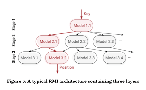
All of this depends of course on being able to train a sufficiently accurate model that can make sufficiently fast predictions, so that the total runtime for Learned Sort, including the training time still beats Radix Sort. For this, the authors use the Recursive Model Index (RMI) architecture as first introduced in ‘The case for learned index structures‘. In brief, RMI uses layers of simple linear models arranged in a hierarchy a bit like a mixture of experts.
During inference, each layer of the model takes the key as an input and linearly transforms it to obtain a value, which is used as an index to pick a model in the next layer.
The main innovation the authors introduce here is the use of linear spline fitting for training (as opposed to e.g. linear regression with an MSE loss function). Spline fitting is cheaper to compute and gives better monotonicity (reducing the time spent in the Insertion Sort phase). Each individual spline model fits worse than its closed-form linear regression counterpart, but the hierarchy compensates. Linear splines result in 2.7x faster training, and up to 35% fewer key swaps during Insertion Sort.
Evaluation
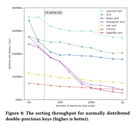
On synthetic datasets containing double-precision keys following a standard normal distribution, the authors compared Learned Sort to a variety of cache-optimized and highly tuned C++ implementations of alternative sorting algorithms, presenting the most competitive alternatives in their results. The following chart shows sorting rates over input dataset sizes varying from one million to one billion items.
Learned Sort outperforms the alternative at all sizes, but the advantage is most significant when the data no longer fits into the L3 cache – an average of 30% higher throughput than the next best algorithm.
The results show that our approach yields an average 3.38x performance improvement over C++ STL sort, which is an optimized Quick- sort hybrid, 1.49x improvement over sequential Radix Sort, and 5.54x improvement over a C++ implementation of Tim- sort, which is the default sorting function for Java and Python.
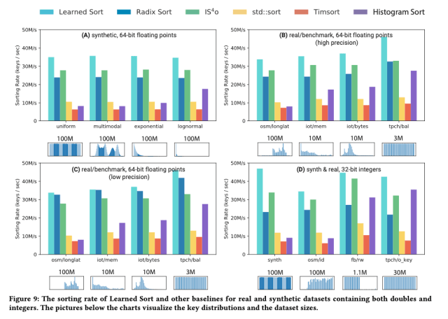
Learned Sort’s advantage holds over real datasets as well (§6.1 for datasets included in the test), and for different element types:
[Learned Sort] results in significant performance improvements as compared to the most competitive and widely used sorting algorithms, and marks an important step into building ML-enhanced algorithms and data structures.
Extensions
The paper also describes several extensions to Learned Sort including sorting in-place, sorting on other key types (strings initially), and improving performance for datasets with many duplicate items.
On the surface this is a paper about fast data ingestion from high-volume streams, with indexing to support efficient querying. As a production system within Microsoft capturing around a quadrillion events and indexing 16 trillion search keys per day it would be interesting in its own right, but there’s a lot more to it than that. Helios also serves as a reference architecture for how Microsoft envisions its next generation of distributed big-data processing systems being built. These two narratives of reference architecture and ingestion/indexing system are interwoven throughout the paper. I’m going to tackle the paper in two parts, focusing today on the reference architecture, and in the next post on the details of Helios itself. What follows is a discussion of where big data systems might be heading, heavily inspired by the remarks in this paper, but with several of my own thoughts mixed in. If there’s something you disagree with, blame me first!
Why do we need a new reference architecture?
Cloud-native systems represent by far the largest, most distributed, computing systems in our history. And the established cloud-native architectural principles behind them aren’t changing here. But zoom out one level of abstraction, and you can also look at cloud platforms as the largest, most-centralised, computing systems in our history. We push as much data processing as possible onto warehouse-scale computers and systems software. It’s a planet-scale client-server architecture with an enormous number of mostly thin clients sharing the services of a few giant server systems. There are several pressures on such a design:
The volume of data continues to grow – by another 2 orders of magnitude this decade according to IDC – as does the velocity of data arrival and the variance in arrival rates. At the same time, end users want results faster – from batch to real-time.
We are observing significant demand from users in terms of avoiding batch telemetry pipelines altogether.
It makes heavy use of comparatively expensive data-center computing facilities
It’s limited by the laws of physics in terms of end-to-end latency
It’s more challenging to build privacy-respecting systems when all data needs to shipped remotely to be processed
The first two of these pressures combine to cause cloud systems to run into one of two limits as exemplified by this quote from the paper:
None of our existing systems could handle these requirements adequately; either the solution did not scale or it was too expensive to capture all the desired telemetry. (Emphasis mine)
Latency limits are one of the drivers pushing us towards more edge computing – a trend which began with static content distribution, then dynamic content (both of which sit on the response path), and now is extending to true edge computation (that can also help improve the request path, e.g. by local processing either eliminating or reducing the amount of data that needs to be sent on to central servers). Industrial IoT use cases are an example here.
The emergence of edge computing has raised new challenges for big data systems… In recent years a number of distributed streaming systems have been built via either open source or industry effort (e.g. Storm, Spark Streaming, MillWheel, Dataflow, Quill). These systems however adopt a cloud-based, centralised architecture that does not include any “edge computing” component – they typically assum an external, independent data ingestion pipeline that directs edge streams to cloud storage endpoints such as Kafka or Event Hubs.
On the privacy front, with increasing awareness and regulation (a good thing, imho!), it’s getting much more complex and expensive to process, store, and secure potentially sensitive data. The most cost-effective mechanism of all is not to store it centrally, and not to process it centrally. Securing data you don’t have and never saw is free! In this regard the machine learning community is ahead of the systems community, with a growing body of work on federated machine learning.
The GDPR directive requires that companies holding EU citizen data provide a reasonable level of protection for personal data… including erasing all personal data upon request… Finding the list of data streams that contain the user’s information requires a provenance graph (as the number of streams is in the order of 10s of billions) and an index (as each stream can span multiple peta-bytes) to avoid expensive linear scans.
What does the new reference architecture look like?
The central idea in the Helios architecture is ’embrace the edge’. Although the word federated doesn’t actually appear in the paper at all, federated big-data systems (c.f. federated machine learning and federated database management systems) seems a reasonable way of describing what’s going on here.
Helios is an effort towards building a new genre of big data systems that combine the cloud and edge as a single, holistic data processing platform.
(And by extension, we could envision end-user devices being part of that holistic platform too).
In the olden days we used to talk about function shipping and data shipping. Function shipping being the idea that you move the compute to the data, and data shipping being the idea that you move the data to the compute. Within todays cloud systems, a lot of function shipping takes place, but for the clients that interact with them, it’s very heavily skewed towards data shipping. In federated big-data systems perhaps the appropriate terms would be function spreading and data spreading. I.e. compute can take place at multiple different points along the path from end device to cloud (and back again), and data can be spread out across layers too. A good guiding principle for designing such a system is probably to minimise data movement – i.e. (1) do as much processing as possible as close to the point of data capture as possible, and only send the aggregated results downstream, and then (2) where pools of data do amass, do as much querying of that data as close to the point of data storage as possible and only send the query results back upstream.
In Helios, this translates to coming up with efficient techniques for splitting computation between end devices, edge, and cloud.
This split has another interesting consequence. We saw earlier that there is end-user pressure to replace batch systems with much lower latency online systems. I observe that computation split across end devices, edge, and cloud doesn’t really sit well with batch processing either. We do distributed batch processing within a layer (e.g. map-reduce) but across layers is different. My conclusion is that federated big-data systems are also online systems. One nice advantage of unifying batch and online processing is that we don’t need to duplicate logic:
This solves the problem of maintaining code that needs to produce the same result in two complex distributed systems.
Generally batch systems have higher throughput and higher latency, and as we reduce the batch size towards online systems, we lower the latency and also the throughput. It will be interesting to watch the throughput characteristics of federated big data systems, but it’s a challenge I think we have to take on. (Helios’ throughput is plenty good enough btw.)
Technically, what might it look like to build a system that works in this way?
Based on our production experience, we posit that a single engine model can (1) enable optimizations such as automatically converting recurring batch queries into streaming queries, dynamically mapping operators/computations to various layers (e.g., end device, edge, cloud), automated A/B testing for figuring out the best query execution plans, join query optimization in multi-tenant scenarios and automatic cost-based view materialisation, and (2) significantly reduce user and operational burden of having to learn and maintain multiple complex stacks.
I’m going to throw one more requirement into the mix for next-generation big data systems. You won’t find this in the Helios paper, but it is something that Microsoft have articulated well in other works, notably Cloudy with a high chance of DBMS: a 10-year prediction for enterprise-grade ML . From a data systems perspective, machine learning is just data processing over (usually) big data sets. We don’t really want completely separate systems for federated machine learning and federated big-data, especially as there are many data cycles between the two (ML both consuming and producing data) and ML is increasingly becoming a mainstream part of many systems and applications. See e.g. the introduction to ‘The case for a learned sorting algorithm.’
The picture that forms in my mind is of a federated differential dataflow style system that processes and materializes just what is needed at each layer. E.g. in the Helios case, “we can similarly distribute the task of data summarization – including filtering, projections, index generation, and online aggregation – to end devices.” One nice thing that falls out of extending such a system all the way out to the end devices is that it means the dataflow engine is effectively responsible for managing all of those pesky caches, and especially cache invalidation.
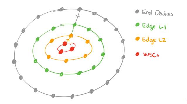
There might be many different layers of edge compute (e.g. 5G base stations, CDN POPs, …) between an end-(user) device and a warehouse scale computer (WSC, aka the cloud). You can think of these as concentric rings forming around WSCs, and conceptually a federated big data system can span all of them.
So far we’ve mostly been talking about spreading compute and data along a single path from an end device to the cloud and back again, leading to a picture like this.
But of course it’s entirely possible (and common) for a node at one layer to interact with multiple nodes at the layer below, leading to a picture more like this:
And furthermore it’s easy to imagine cases where peer-to-peer communication between nodes at the same level also makes sense:
In general we’re looking at a dynamic dataflow topology with very large numbers of nodes.
Helios is a successful production example of a subset of these ideas, and we’ll look at Helios itself in much more detail in the next post. For now I’ll close with this thought:
Helios provides one example for a specific type of computation, i.e. indexing of data. There are a number of related problems, such as resource allocation, query optimization, consistency, and fault tolerance. We believe that this is a fertile ground for future research.
Last time out we looked at the motivations for a new reference blueprint for large-scale data processing, as embodied by Helios. Today we’re going to dive into the details of Helios itself. As a reminder:
Helios is a distributed, highly-scalable system used at Microsoft for flexible ingestion, indexing, and aggregation of large streams of real-time data that is designed to plug into relationals engines. The system collects close to a quadrillion events indexing approximately 16 trillion search keys per day from hundreds of thousands of machines across tens of data centres around the world.
As an ingestion and indexing system, Helios separates ingestion and indexing and introduces a novel bottoms-up index construction algorithm. It exposes tables and secondary indices for use by relational query engines through standard access path selection mechanisms during query optimisation. As a reference blueprint, Helios’ main feature is the ability to move computation to the edge.
Requirements
Helios is designed to ingest, index, and aggregate large streams of real-time data (tens of petabytes a day). For example, the log data generated by Azure Cosmos. It supports key use cases such as finding records relating to specific attributes (e.g. for incident support), impact and drill-down analysis, and performance monitoring and reporting. One interesting use case is in support of GDPR right to be forgotten requests, where it becomes necessary to search 10s of billions of streams to find those containing a user’s information.
Incoming streams can have data rates as high as 4TB/minute, with many columns to be indexed (7+ is common) and high cardinality.
System design
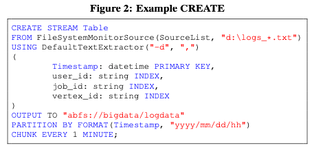
A stream table is defined by a loose schema which defines the sources to be monitored (as a SourceList) and indices to be created. For example:
Based on the CREATE STREAM statement, Helios generates an agent executable to be deployed on every machine producing a log that is part of the stream. It also generates an executable to be run on the server-side ingestion machines. The agent process accumulates and chunks incoming data into data blocks (with frequency determined by the CHUNK EVERY clause). Optionally, and central to how Helios handles high volume and velocity ingest at manageable scale and cost, the agent can also perform local processing (parsing, indexing, and aggregation) and send the resulting index entries to the ingestion clusters in a compact format.
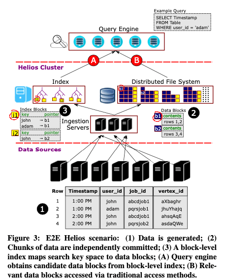
Ingestion servers are stateless, running the user-defined dataflow (based on the CREATE SCHEMA statement) to process incoming blocks. Data blocks are stored in a distributed file system, and once acknowledged by the file system, an entry is written into Helio’s progress log. The progress log is used to track the progress of both data ingestion and index building. Secondary index generation (hydration) then happens asynchronously. The resulting index blocks are merged into a global index which maps (column, value) pairs to data block URIs.
The progress log is the only strongly synchronized component in Helios, and is deployed in quorum based rings of 5 servers. There are multiple replicated logs each governing a partition of the data set. In this manner Helios achieves a consistent rate of 55,000 writes/second for metadata persistence.
Indexing
A key factor in Helios’s success is asynchronous index mangement: Helios maintains eventually consistent indexes against the data, but exposes a strongly consistent queryable view of the underlaying data with best-effort index support.
Helios’ index is a multi-level (tree-based) structure that is built in a bottom-upmanner. I.e., information is inserted at the leaves, and the index then ‘grows upwards’ through merge and add operations. The authors point out an interesting similarity to learned index structures here: “At the highest level, a learned index tries to learn a function that maps an index search key to the leaf nodes containing the search key. The Helios structure in its generic form performs exactly the same function, with the different that the mapping is not learned from data but composed from the (typically, hash) partitioning functions used by the different index levels.“
Indexing begins by scanning the progress log from the latest checkpoint, with an initial leaf node at the bottom of the tree (level 0) constructed for each chunk. No global order is imposed here, indexed keys are simply packed into leaf nodes based on arrival order. Multiple nodes at the same level may be combined into one using the merge operator in accordance with a merge policy. Just as level 0 watches blocks arrive in the progress log and follows along creating leaf nodes, so the next level up, level 1 watches the progress of leaf nodes arriving at level 0, and creates a higher level index over the leaf nodes by applying the add operator. Level 2 follows the progress of level 1 in a similar manner, and so on for the desired number of levels. The result is an indexing frontier that moves forward across the levels through a per-level watermark.
An index node is a collection of (key, pointers) pairs. The merge operation combines two index nodes and by taking the union of their keys, and for each key the union of the pointers. E.g. if and then . Helios uses a size-based merge policy in which two nodes are merged if they are both below a given size threshold.
The add operation creates a new node at one level up containing the union of the keys in the blocks being added, and pointers to the nodes in the level below containing entries for those keys. E.g. . Helios also uses a size-based add policy, in which nodes are added (at higher and higher levels) until the size of the resulting node reaches a configurable threshold.
Note that the resulting structure may contain orphan nodes (shown in grey in the figure above) that do not have any parent in the layer above. This has implications for query processing that we’ll look at shortly.
Index compaction, which also takes place bottom-up, is triggered when a configurable number of data blocks have been processed.
Federated indexing
Our initial approach towards data and index management focused towards bringing in data from all the sources into an ingestion cluster and performing the required post-processing operations (e.g. parsing, indexing, etc.). However, this approach incurs significant costs… The hierarchical/recursive indexing model gives the freedom of distributing our computation acress the agents and ingestion back-end servers, sharing the same intuition as the current trend of edge computation.
Pre-processing on agents reduces the size of the ingestion cluster required, at the cost of consuming processing power on the source machine. In Helios production deployments, the agent typically consumes 15%-65% of a single CPU core, and stays under an allocated memory budget of 1.6GB. The generated agent and ingestion code utilises a shared library called Quarkwhich provides a selection of parsers, extractors, indexers, partitioners, serializers and compressors as well as query-processing operators with predicate push-down.
Querying
Helios indexes are represented and exposed as data in easily accessible formats, available for any query engine. This allows us to democratise index usage outside of Helios, e.g. query engines can perform their own cost-based index access path selection, and index reads can independently scale without being constrained by compute resources provided by Helios. In fact, we were able to integrate Apache Spark with no changes to its optimizer/compiler.
Due to the existence of orphan nodes, querying can’t proceed in a pure top-down manner. So Helios provides a hybrid index scan operator. Querying starts by moving down the tree from the root nodes (which are orphan nodes by definition), and then recursively repeating this process for each of the orphan nodes at the next level down moving right.
In Figure 6 above for example, we can search down the tree from , but in doing so we miss any potential hits in the orphan node at the next level down. So after processing we start a new search from . This in turn may miss hits in the orphan block so we then drop-down once more and move right…
Helios in production
Helios has multiple uses at Microsoft including supporting debugging and diagnostics, workload characterization, cluster health monitoring, deriving business insights, and performing impact analysis.
Helios clusters have been in production for the last five years, collecting close to a quadrillion log lines per day from hundreds of thousands of machines spread across tens of datacenters.
Before we dive into this paper, if you click on the link above and then download and open up the paper pdf you might notice the familiar red/orange splash of USENIX, and appreciate the fully open access. USENIX is a nonprofit organisation committed to making content and research freely available – both conference proceedings and the recorded presentations of their events. Without in-person conferences this year, income is down and events are under threat. If you want to help them, you have options to donate, become a member, or even talk to your organisation about becoming a partner, benefactor, or patron. Every little helps!
Back in 2017 the engineering team at Facebook had a problem. They needed a table store to power core control plane services, which meant strong guarantees on durability, consistency, and availability. They also needed it fast – the goal was to be in production within 6 to 9 months. While ultimately this new system should be able to take advantage of the latest advances in consensus for improved performance, that’s not realistic given a 6-9 month in-production target. So realistically all that could be done was to choose an existing consensus implementation and integrate it. Integrating an existing implementation brings problems of its own though:
Laying the system over an existing shared log such as LogDevice would allow us to reach production quickly, but also tie us for perpetuity to the fault-tolerance and performance properties of that consensus implementation.
What Facebook needed, literally, was a plan to throw one away. I.e., a plan that let them get into production quickly with an existing implementation, and then be able to upgrade it later without disturbing system operation (nobody wants to take down the central control plane for maintenance!). This calls for the oldest tool in the box: a level of indirection. In other words, an API based abstraction over consensus, together with a runtime that supports hot-swapping of those implementations. The standout candidate as the API for consensus is the shared log.
Recently, the shared log has gained traction as an API for consensus in research and industry. Applications can replicate state via this API by appending updates to the shared log, checking its tail, and reading back updates from it. The consensus protocol is hidden behind the shared log API, allowing applications to bind to any implementation at deployment time.
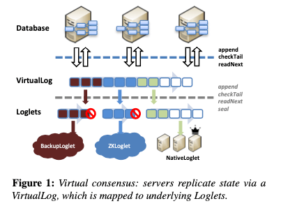
Behind the shared log API is a log abstraction that maps log positions to log entries. If you think of this a bit like mapping memory addresses to data in memory, then another parallel comes to mind: the virtual address space. One logical log, but with different portions of the log address space mapped to different backing shared log instances. This is the core idea in Delos, a VirtualLog that virtualises consensus.
We propose the novel abstraction of a virtual shared log (or VirtualLog). The VirtualLog exposes a conventional shared log API; applications above it are oblivious to its virtualized nature. Under the hood, the VirtualLog chains multiple shared log instances (called Loglets) into a single shared log.
It’s such a powerful idea that I can imagine distributed systems implementers everywhere adopting it from now on. What does the VirtualLog give us?
Firstly, it solves the upgrade problem. We have an existing Loglet writing log entries into the address space. To upgrade, the portion of the address space managed by this Loglet is sealed to prevent further writes, and then the Loglet chain is reconfigured to add the new Loglet at the tail. That’s not just theoretical, Facebook actually did this in production while Delos was processing over 1.8 billion transactions per day. The initial version of Delos went into production after eight months using a ZooKeeper-backed Loglet implementation, and then four months later it was swapped out for a new custom-built NativeLoglet that gave a 10x improvement in end-to-end latency.
Once you have a trusted reconfiguration protocol to move from one Loglet chain configuration to another, you can do lots of interesting things. For example, Loglets might be instances of the same ordering protocol, but with different parameters, or they could be entirely different log implementations (e.g. replacing Paxos with Raft), or they could be shims over external storage systems. If you have an existing implementation with its own leader elections, internal reconfiguration, and epochs that can sit happily under the Loglet abstraction. But critically, Loglets no longer need to handle all of that complexity:
While the VirtualLog’s reconfiguration mechanism can be used solely for migrating between entirely different Loglet implementations, it can also switch between different instances of the same Loglet protocol with changes to leadership, roles, parameters, and membership. As a result, the Loglet itself can be a statically configured protocol, without any internal support for reconfiguration. In fact, the Loglet does not even have to implement fault-tolerant consensus (i.e. be highly available for appends via leader election), as long as it provides a fault tolerant seal command, which is theoretically weaker and simpler to implement.
This separation of concerns moves reconfiguration into the VirtualLog control plane, leaving Loglets responsible for the data plane. It makes reconfiguration easier as well as simplifying the implementation of Loglets. If a Loglet fails for appends, it is simply sealed and the VirtualLog switches to a new Loglet.
Sealing
A minimal Loglet needs to provide totally ordered, durable storage via the shared log API. It can do this within a static configuration with no support for role or membership changes and no leader election. What it must provide however, is a highly available seal command that prevents any new appends from being acknowledged.
Once sealed, a Loglet can never be unsealed. So we have a couple of handy properties that make implementing seal much easier than a general purpose highly available append: only one value can ever be proposed, and that value is sticky. In Facebook’s implementation of NativeLoglet, seal simply sets a bit on a quorum of servers.
In addition to seal, a minimal Loglet is also responsible for its own failure detection, asking the VirtualLog to reconfigure when a failure is detected, and supplying a new Loglet configuration minus the failed servers.
Reconfiguration
Existing consensus systems often store the configuration and epoch information inline in the same totally ordered log as other commands. For VirtualLog, that would mean writing the configuration for the new Loglet inside the log address space of the outgoing Loglet before it is sealed. And that would put more complexity onto Loglets, requiring them to be highly available for appends, not just seal.
The VirtualLog uses a separate MetaStore instead, whose job is to manage the configuration of the VirtualLog over time. Because reconfiguration happens less frequently than regular command sequencing, the consensus protocol for reconfiguration can favour simplicity over out-and-out performance. For Facebook’s Delos, reconfiguration latencies of 10s of ms are ok.
The MetaStore exposes a single versioned register supporting a conditional write: writing requires supplying a new value and an expected existing version. Any client can initiate a reconfiguration, or complete a reconfiguration begun by another client. Reconfiguration has three steps:
The client seals the current chain by sealing its active segment. A call to checkTail will now return the start of a new active segment. This is an idempotent operation.
The reconfiguring client writes a new chain to the MetaStore. Because of the conditional write, if multiple clients are racing to reconfigure, at most one one can win.
The reconfiguring client fetches the new chain from the MetaStore (in the case where its write failed in step 2).
Clients trying to write to the old active segment after step 1 will receive a ‘sealed’ error code, and can retry after fetching the latest chain from the MetaStore.
The NativeLoglet
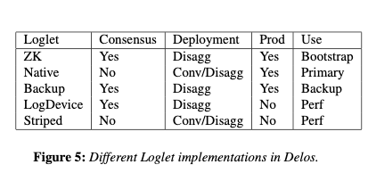
Delos currently supports three disaggregated Loglets acting as shims over external services (ZooKeeper, a LogDevice service, and a Backup service used for cold storage). It also has two of its own Loglet implementations that can be run either converged or disaggregated: the NativeLoglet and the StripingLoglet.
In production, Facebook use the NativeLoglet in converged form. NativeLoglet implements seal by setting a bit on a quorum of servers. It uses a a central sequencer to assign positions to commands and forward requests to LogServers. An append is considered globally committed once a majority acknowledge. If the sequencer fails, NativeLoglet simply becomes unavailable for appends.
Practically, we found this protocol much easier to implement than fault-tolerant consensus: it took just under 4 months to implement and deploy a production-quality native Loglet.
Striping Loglets
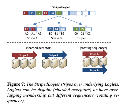
The StripedLoglet is where things start to get even more interesting. A StripedLoglet is responsible for one portion of the global log address space, but internally it further maps (stripes) that portion over multiple nested Loglets.
This provides a simple way (about 300 loc) to scale throughput. For example, a shared sequencer bottleneck can be relieved by introducing a rotating sequencer – multiple sequencers dividing an address space between them and sharing the same underling LogServers. Alternatively, the address space can mapped to multiple underlying LogServer clusters to increase throughput.
Even though it is a composite, a StripedLoglet must still be sealed as a whole even if only one of its stripes needs to be reconfigured.
Delos in production
The evaluation section has lots of good information on experiences running Delos in production, as well as some synthetic benchmarks. The in-production switch from a ZK Loglet to NativeLoglet was done for the first time on April 2nd 2019, and gave a 10x improvement at p99 for gets, and a 5x improvement for writes.
My favourite example here is a really cool use case for reconfiguration. Most of the time Delos runs with a converged Loglet implementation, since this reduces the external dependencies of a very critical system. Under a log spike though, it can be reconfigured to run with a disaggregated Loglet, giving higher throughput. A related example is when Delos is running in converged mode and e.g. two of the five converged database replicas crash. Now the database and the shared log are fate-sharing and at risk if one more node is lost…
In this situation (which was not uncommon), we found it valuable to reconfigure the system to a disaggregated log, temporarily decoupling the fate of the database and the log. Once the database was restored to five replicas, we reconfigured back.
The overheads of virtualisation are pleasingly low: about 100-150µs at p99 latency, 10s of ms for reconfiguration, and no impact on peak throughput.
Limitations and future work
It all sounds pretty amazing doesn’t it! There are a couple of limitations: (1) consensus protocols that exploit speculation or commutativity don’t currently fit under the Loglet API. “In future work, we plan to extend virtual consensus to partially ordered shared logs.”, and (2) there’s a latency hit for VirtualLog-driven reconfiguration which may or may not be important in your scenario.

 Video is a core data path across NVIDIA Jetson applications, from robotics and intelligent video analytics to industrial automation, healthcare, media…
 AI infrastructure spans multiple layers, from compute and networking to storage, orchestration, and applications. When performance degrades, identifying the…
 Alibaba released the open weights for Qwen3.8-2.4T-A95B (Qwen3.8-Max), its largest open-weight model, bringing near-frontier capabilities to the open…
 Teams customize their models to hit their targets for latency, speed, memory, and compute. With the open NVIDIA Nemotron family of models, developers can find…
 Uniform Manifold Approximation and Projection (UMAP) is a dimensionality reduction technique widely used for visualization and feature extraction. Applications…
 Atomistic simulation requires three things: knowledge of the science, compute-efficient implementation of simulations, and accessible interfaces to the…
 be the number of buckets (
 is reached. If at any stage a model prediction places in an item in a bucket that is already full, this item is just moved to a spill bucket instead.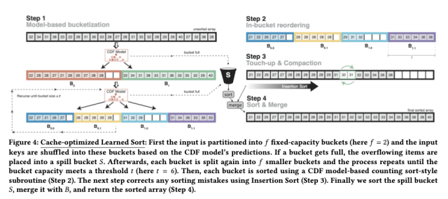



 and
and  by taking the union of their keys, and for each key the union of the pointers. E.g. if
  and
and  then
then  . Helios uses a size-based merge policy in which two nodes are merged if they are both below a given size threshold.
 . Helios also uses a size-based add policy, in which nodes are added (at higher and higher levels) until the size of the resulting node reaches a configurable threshold.
 , but in doing so we miss any potential hits in the orphan node
  at the next level down. So after processing
  so we then drop-down once more and move right…