Demand for real-time insights and autonomous decision-making is growing in various industries. To meet this demand, we need scalable edge-solution platforms…
Demand for real-time insights and autonomous decision-making is growing in various industries. To meet this demand, we need scalable edge-solution platforms that can effectively process AI-enabled sensor data right at the source and scale out to on-premises or cloud compute resources.
However, developers face many challenges in using AI and sensor processing at the edge:
Real-time latency requirements
The complexity of building and maintaining custom pipelines for AI-enabled sensor processing
The need for hardware-agnostic solutions to meet heterogeneous hardware needs at the edge
Multimodality and processing of various sensory modalities
Integration from edge to on-premises to a cloud-distributed network
Long-term whole-stack stability
Before NVIDIA Holoscan, no singular platform offered a comprehensive solution that effectively addressed the multitude of edge AI challenges. By seamlessly integrating data movement, accelerated computing, real-time visualization, and AI inferencing, Holoscan ensures optimal application performance. It abstracts away complexities for developers, reduces time to market, and offers the convenience of coding in Python and C++, all in a low-code, high-performance infrastructure.
“The Holoscan platform enables new SaMD (software as a medical device) to be quickly productized with seamless integration with the development environment to enable SaMD productization and fast-track deployment,” said Nhan Ngo Dinh, president of Cosmo Intelligent Medical Devices. “This accelerates the time to market with integrated development programmable using the NVIDIA Holoscan SDK, easy to transition from development to production.”
For edge developers, navigating the heterogeneous landscape of edge devices with varying hardware requirements and architectures can be daunting. Holoscan simplifies this complexity through its hardware-agnostic approach.
The platform provides a unified stack, accommodating a wide range of devices from x86 to aarch64 and NVIDIA Jetson Orin AGX to NVIDIA IGX Orin, catering to different power, size, cost, compute, and configuration needs. This versatility liberates you from hardware constraints while promoting interoperability, maintainability, and scalability across applications.
The v0.6 release of NVIDIA Holoscan introduces new features that empower you to reach new levels of scalability, productivity, and ease of use when building AI-streaming solutions. Specifically, this new set of features enables the following benefits:
Scalability at the edge through a distributed computing architecture
Portability, collaboration, and interoperability for platform development
Advanced profiling with data frame flow tracking for optimal performance
Scalability through distributed computing architecture
For developers with heavy workloads or interested in scaling up and out, the Holoscan v0.6 multi-GPU, multi-node support enables distributed computing. Specifically, you can now deploy distributed applications and use all the resources available on the edge with multiple GPUs on a single node. Or you can deploy a single Holoscan application on separate physical nodes with optimized network communication.
Multi-GPU, multi-node enables sensor processing applications to scale with ever-increasing compute requirements and grants you more flexibility and scalability in your designs. For users, it opens new possibilities with increased processing power, parallel processing, separating workloads based on criticality, post-deployment scale-up without replacing existing units, fault tolerance, and reliability.
Figure 1. Distributed applications scaled out with multi-fragment APIs
Portability, collaboration, and interoperability for platform developers
If you are developing a platform instead of creating standalone products from scratch, Holoscan v0.6 provides a set of new features enabling more scalability and flexibility for broader use and ease of integration:
App packager: Grants portability through the easy containerization and deployment of the apps, enhancing collaboration and contributions to the platform.
Multi-backend: Streamlines the transition from model training to AI app building enabled by the plug-and-play deployment of already trained PyTorch models.
Holoviz volumetric rendering: Provides built-in volumetric rendering in support of medical imaging visualization.
Advanced profiling with data frame flow tracking
The upcoming release includes a data frame flow tracking feature that enables you to measure performance through data frame tracking so that you can quickly adjust bottlenecks. In addition, the new multithreaded scheduler enables applications to run operators in parallel. As a result, the applications have optimized the use of system resources.
Use cases and success stories
The NVIDIA Holoscan SDK has rapidly evolved into an accelerated, full-stack infrastructure, making significant contributions to scalable, software-defined, and real-time processing across various domains.
The following healthcare companies have embraced and built on this technology:
Medtronic, the largest medical device company in the world, is building a next-generation AI-assisted colonoscopy system (pending FDA approval) on the Holoscan platform.
Moon Surgical, a Paris-based robotic surgery company, is finalizing the productization of Maestro, an accessible, adaptive surgical-assistant robotics system built on Holoscan and IGX.
ORSI Academy, a surgical training center in Belgium, has used Holoscan to support first-in-human real-world, robot-assisted surgery for critical operations like the removal of cancerous kidneys.
“Holoscan abstracts away the challenges in building safe and reliable sensor data processing pipelines for medical device applications. Traditionally such pipelines required dedicated teams of specialists to develop and maintain,” said David Noonan, CTO at Moon Surgical. Using Holoscan, we’re able to launch innovative features for our Maestro surgical robotics system with short development timelines while maintaining a lean R&D team.”
Other use cases include AR/VR, radar technology, and scientific instrumentation.
Magic Leap is working on a Holoscan-based solution that combines AI with true augmented reality to revolutionize physician and surgeon training, visualization, and complex procedure performance.
Researchers from the Georgia Tech Research Institute used Holoscan to develop a real-time radar application used in defense, aerospace, meteorology, navigation, and surveillance.
NVIDIA and Analog Devices collaborated to build a 5G Instrumentation application that leverages Holoscan for compute-intensive signal processing at over 120 Gbps on the NVIDIA IGX platform.
At Diamond Light Source, a world-renowned synchrotron in the UK, developers used Holoscan and Jax-based Holoscan operators to easily connect Holoscan to existing Ptychography software libraries to speed up image processing and reconstruction.
“With Holoscan, we’ve created an end-to-end data streaming pipeline that enables live ptychographic image processing at the I08-1 beam line, considerably enriching the overall user interaction,” said Paul Quinn, Imaging and Microscopy Science group leader, Diamond Light Source.
Get started with Holoscan 0.6
The release of NVIDIA Holoscan 0.6 marks a significant milestone in the development of edge AI solutions, offering unprecedented scalability, flexibility, and performance. With its diverse range of applications and success stories, Holoscan is shaping the future of AI-enabled sensor processing at the edge, opening new possibilities for various industries worldwide.
Deep neural networks (DNNs) are the go-to model for learning functions from data, such as image classifiers or language models. In recent years, deep models…
Deep neural networks (DNNs) are the go-to model for learning functions from data, such as image classifiers or language models. In recent years, deep models have become popular for representing the data samples themselves. For example, a deep model can be trained to represent an image, a 3D object, or a scene, an approach called Implicit Neural Representations. (See also Neural Radiance Fields and Instant NGP). Read on for a few examples of performing operations on a pretrained deep model for both DNNs-that-are-functions and DNNs-that-are-data.
Suppose you have a dataset of 3D objects represented using Implicit Neural Representations (INRs) or Neural Radiance Fields (NeRFs). Very often, you may wish to “edit” the objects to change their geometry or fix errors and abnormalities. For example, to remove a handle of a cup or make all car wheels more symmetric than was reconstructed by the NeRF.
Unfortunately, a major challenge with using INRs and NeRFs is that they must be rendered before editing. Indeed, editing tools rely on rendering the objects and directly fine-tuning the INR or NeRF parameters. See, for example, 3D Neural Sculpting (3DNS): Editing Neural Signed Distance Functions. It would have been much more efficient to change the weights of the NeRF model directly without rendering it back to 3D space.
As a second example, consider a trained image classifier. In some cases, you may want to apply certain transformations to the classifier. For example, you may want to take a classifier trained in snowy weather and make it accurate for sunny images. This is an instance of a domain adaptation problem.
However, unlike traditional domain adaptation approaches, the setting focuses on learning the general operation of mapping a function (classifier) from one domain to another, rather than transferring a specific classifier from the source domain to the target domain.
Neural networks that process other neural networks
The key question our team raises is whether neural networks can learn to perform these operations. We seek a special type of neural network “processor” that can process the weights of other neural networks.
This, in turn, raises the important question of how to design neural networks that can process the weights of other neural networks. The answer to this question is not that simple.
Figure 1. Two examples of data-specialized architectures: convolutional neural networks for images and DeepSets for point clouds
Previous work on processing deep weight spaces
The simplest way to represent the parameters of a deep network is to vectorize all weights (and biases) as a simple flat vector. Then, apply a fully connected network, also known as a multilayer perceptron (MLP).
Unfortunately, this approach has a major shortcoming because the space of neural network weights has a complex structure (explained more fully below). Applying an MLP to a vectorized version of all parameters ignores that structure and, as a result, hurts generalization. This effect is similar to other types of structured inputs, like images. This case works best with a deep network that is not sensitive to small shifts of an input image.
The solution is to use convolutional neural networks. They are designed in a way that is largely “blind” to the shifting of an image and, as a result, can generalize to new shifts that were not observed during training.
Here, we want to design deep architectures that follow the same idea, but instead of taking into account image shifts, we want to design architectures that are not sensitive to other transformations of model weights, as we describe below.
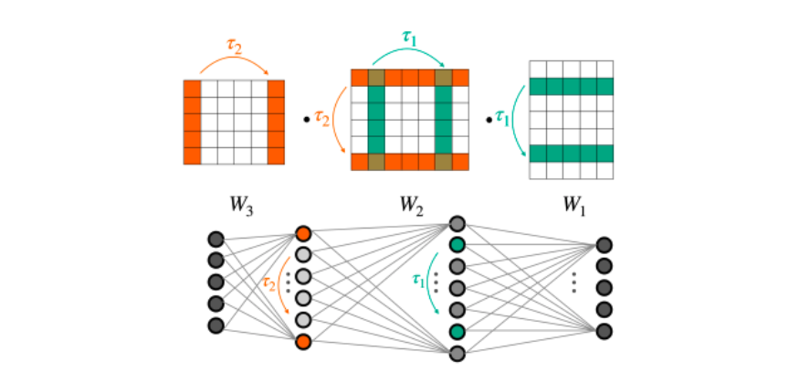
Specifically, a key structural property of neural networks is that their weights can be permuted while they still compute the same function. Figure 2 illustrates this phenomenon. This important property is overlooked when applying a fully connected network to vectorized weights.
Figure 2. The weight symmetries (top) of a multilayer perceptron (MLP) with two hidden layers (bottom). Changing the order of neurons in internal layers preserves the function represented by the MLP
Unfortunately, a fully connected network that operates on flat vectors sees all these equivalent representations as different. This makes it much harder for the network to generalize across all such (equivalent) representations.
A brief introduction to symmetries and equivariant architectures
Fortunately, the preceding MLP limitations have been extensively studied in a subfield of machine learning called Geometric Deep Learning (GDL). GDL is about learning objects while being invariant to a group of transformations of these objects, like shifting images or permuting sets. This group of transformations is often called a symmetry group.
In many cases, learning tasks are invariant to these transformations. For example, finding the class of a point cloud should be independent of the order by which points are given the network because that order is irrelevant.
In other cases, like point cloud segmentation, every point in the cloud is assigned a class to which part of the object it belongs to. In these cases, the order of output points must change in the same way if the input is permuted. Such functions, whose output transforms according to the input transformation, are called equivariant functions.
More formally, for a group of transformations G, a function L: V → W is called G-equivariant if it commutes with the group action, namely L(gv) = gL(v) for all v ∈ V, g ∈ G. When L(gv) = L(v) for all g∈ G, L is called an invariant function.
In both cases, invariant and equivariant functions, restricting the hypothesis class is highly effective, and such symmetry-aware architectures offer several advantages due to their meaningful inductive bias. For example, they often have better sample complexity and fewer parameters. In practice, these factors result in significantly better generalization.
Symmetries of weight spaces
This section explains the symmetries of deep weight spaces. One might ask the question: Which transformations can be applied to the weights of MLPs, such that the underlying function represented by the MLP is not changed?
One specific type of transformation, called neuron permutations, is the focus here. Intuitively, when looking at a graph representation of an MLP (such as the one in Figure 2), changing the order of the neurons at a certain intermediate layer does not change the function. Moreover, the reordering procedure can be done independently for each internal layer.
In more formal terms, an MLP can be represented using the following set of equations:
The weight space of this architecture is defined as the (linear) space that contains all concatenations of vectorized weights and biases . Importantly, in this setup, the weight space is the input space to the (soon-to-be-defined) neural networks.
So, what are the symmetries of weight spaces? Reordering the neurons can be formally modeled as an application of a permutation matrix to the output of one layer and an application of the same permutation matrix to the next layer. Formally, a new set of parameters can be defined by the following equations:
The new set of parameters is different, but it is easy to see that such transformations do not change the function represented by the MLP. This is because the two permutation matrices and cancel each other (assuming an elementwise activation function like ReLU).
More generally, and as stated earlier, a different permutation can be applied to each layer of the MLP independently. This means that the following more general set of transformations will not change the underlying function. Think about these as symmetries of weight spaces.
Most equivariant architectures in the literature follow the same recipe: a simple equivariant layer is defined, and the architecture is defined as a composition of such simple layers, possibly with pointwise nonlinearity between them.
When the task at hand is invariant, it is possible to add an invariant layer on top of the equivariant layers with an MLP, as illustrated in Figure 3.
Figure 3. A typical equivariant architecture composed of several simple equivariant layers, followed by an invariant layer and a fully connected layer
We follow this recipe in our paper, Equivariant Architectures for Learning in Deep Weight Spaces. Our main goal is to identify simple yet effective equivariant layers for the weight-space symmetries defined above. Unfortunately, characterizing spaces of general equivariant functions can be challenging. As with some previous studies (such as Deep Models of Interactions Across Sets), we aim to characterize the space of all linear equivariant layers.
We have developed a new method to characterize linear equivariant layers that is based on the following observation: the weight space V is a concatenation of simpler spaces that represent each weight matrix V=⊕Wi. (Bias terms are omitted for brevity).
This observation is important, as it enables writing any linear layer as a block matrix whose (i,j)-th block is a linear equivariant layer between and . This block structure is illustrated in Figure 4.
But how can we find all instances of ? Our paper lists all the possible cases and shows that some of these layers were already characterized in previous work. For example, for internal layers was characterized in Deep Models of Interactions Across Sets.
Remarkably, the most general equivariant linear layer in this case is a generalization of the well-known deep sets layer that uses only four parameters. For other layers, we propose parameterizations based on simple equivariant operations such as pooling, broadcasting, and small fully connected layers, and show that they can represent all linear equivariant layers.
Figure 4 shows the structure of L, which is a block matrix between specific weight spaces. Each color represents a different type of layer. are in red. Each block maps a specific weight matrix to another weight matrix. This mapping is parameterized in a way that relies on the positions of the weight matrices in the network.
Figure 4. The block structure of the proposed linear equivariant layer
The layer is implemented by computing each block independently and then summing the results for each row. Our paper covers some additional technicalities, like processing the bias terms and supporting multiple input and output features.
We call these layers Deep Weight Space Layers (DWS Layers), and the networks constructed from them Deep Weight Space Networks (DWSNets). We focus here on DWSNets that take MLPs as input. For more details on extensions to CNNs and transformers, see Appendix H in Equivariant Architectures for Learning in Deep Weight Spaces.
The expressive power of Deep Weight Space Networks
Restricting our hypothesis class to a composition of simple equivariant functions may unintentionally impair the expressive power of equivariant networks. This has been widely studied in the graph neural networks literature cited above. Our paper shows that DWSNets can approximate feed-forward operations on input networks—a step toward understanding their expressive power. We then show that DWS networks can approximate certain “nicely behaving” functions defined in the MLP function space.
Experiments
DWSNets are evaluated in two families of tasks. First, taking input networks that represent data, like INRs. Second, taking input networks that represent standard I/O mappings such as image classification.
Experiment 1: INR classification
This setup classifies INRs based on the image they represent. Specifically, it involves training INRs to represent images from MNIST and Fashion-MNIST. The task is to have the DWSNet recognize the image content, like the digit in MNIST, using the weights of these INRs as input. The results show that our DWSNet architecture greatly outperforms the other baselines.
Table 1. With INR classification, the class of an INR is defined by the image that it represents (average test accuracy)
Importantly, classifying INRs to the classes of images they represent is significantly more challenging than classifying the underlying images. An MLP trained on MNIST images can achieve near-perfect test accuracy. However, an MLP trained on MNIST INRs achieves poor results.
Experiment 2: Self-supervised learning on INRs
The goal here is to embed neural networks (specifically, INRs) into a semantic coherent low-dimensional space. This is an important task, as a good low-dimensional representation can be vital for many downstream tasks.
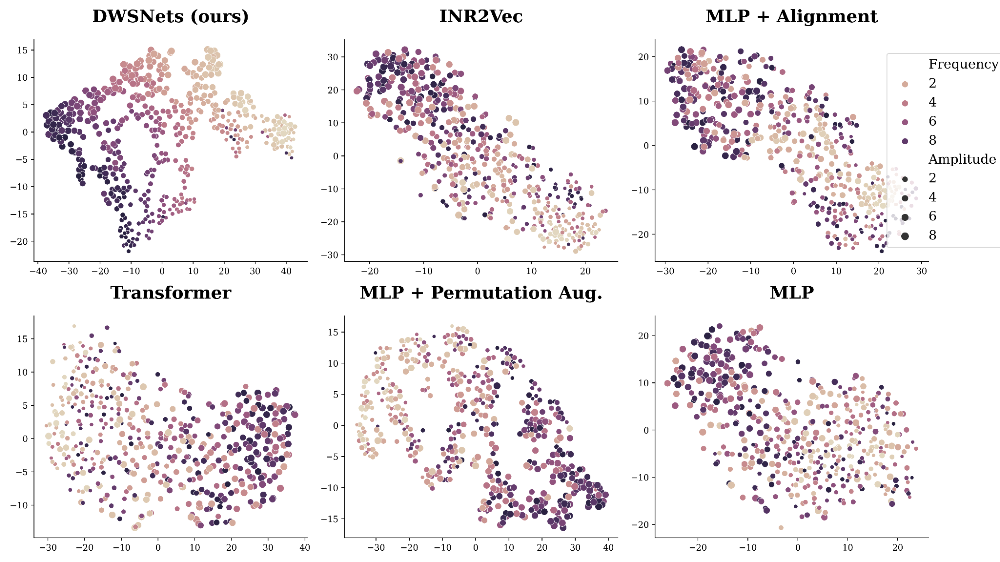
Our data consists of INRs fitted to sine waves of the form asin(bx), where a, b are sampled from a uniform distribution on the interval [0,10]. As the data is controlled by these two parameters, the dense representation should extract this underlying structure.
Figure 5. TSNE embeddings of input MLPs obtained by training using self-supervision
A SimCLR-like training procedure and objective are used to generate random views from each INR by adding Gaussian noise and random masking. Figure 4 presents a 2D TSNE plot of the resulting space. Our method, DWSNet, nicely captures the underlying characteristics of the data while competing approaches struggle.
Experiment 3: Adapting pretrained networks to new domains
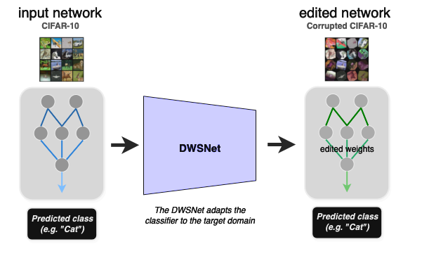
This experiment shows how to adapt a pretrained MLP to a new data distribution without retraining (zero-shot domain adaptation). Given input weights for an image classifier, the task is to transform its weights into a new set of weights that performs well on a new image distribution (the target domain).
At test time, the DWSnet receives a classifier and adapts it to the new domain in a single forward pass. The CIFAR10 dataset is the source domain and a corrupted version of it is the target domain (Figure 6).
Figure 6. Domain adaptation using DWSNets
The results are presented in Table 2. Note that at test time the model should generalize to unseen image classifiers, as well as unseen images.
Table 2. Adapting a network to a new domain. Test accuracy of CIFAR-10-Corrupted models adapted from CIFAR-10 models
Future research directions
The ability to apply learning techniques to deep-weight spaces offers many new research directions. First, finding efficient data augmentation schemes for training functions over weight spaces has the potential to improve DWSNets generalization. Second, it is natural to study how to incorporate permutation symmetries for other types of input architectures and layers, like skip connections or normalization layers. Finally, it would be useful to extend DWSNets to real-world applications like shape deformation and morphing, NeRF editing, and model pruning. Read the full ICML 2023 paper, Equivariant Architectures for Learning in Deep Weight Spaces.
NVIDIA interns around the globe wrapped up a week of “Our Founders Edition” celebrations — a nod to a special line of GeForce cards — which featured company lore and talks from founders Jensen Huang and Chris Malachowsky. Read article >
NVIDIA Jetson Orin is the best-in-class embedded AI platform. The Jetson Orin SoC module has the NVIDIA Ampere architecture GPU at its core but there is a lot…
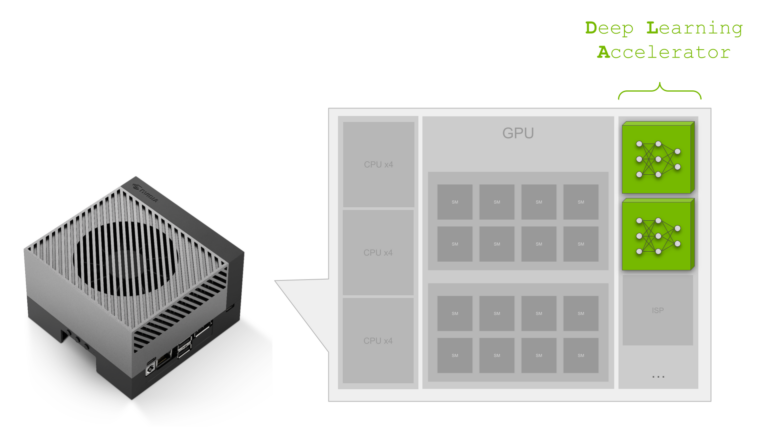
NVIDIA Jetson Orin is the best-in-class embedded AI platform. The Jetson Orin SoC module has the NVIDIA Ampere architecture GPU at its core but there is a lot more compute on the SoC:
A dedicated deep learning inference engine in the Deep Learning Accelerator (DLA) for deep learning workloads
The Programmable Vision Accelerator (PVA) engine for image processing and computer vision algorithms
The Multi-Standard Video Encoder (NVENC) and Multi-Standard Video Decoder (NVDEC)
The NVIDIA Orin SoC is powerful, with 275 peak AI TOPs, making it the best embedded and automotive AI platform. Did you know that almost 40% of these AI TOPs come from the two DLAs on NVIDIA Orin? While NVIDIA Ampere GPUs have the best-in-class throughput, the second-generation DLA has the best-in-class power efficiency. As applications of AI have rapidly grown in recent years, so has the demand for more efficient computing. This is especially true on the embedded side where power efficiency is always a key KPI.
That’s where DLA comes in. DLA is designed specifically for deep learning inference and can perform compute-intensive deep learning operations like convolutions much more efficiently than a CPU.
When integrated into an SoC as on Jetson AGX Orin or NVIDIA DRIVE Orin, the combination of GPU and DLA provides a complete solution for your embedded AI applications. In this post, we discuss the Deep Learning Accelerator to help you stop missing out. We cover a couple of case studies in automotive and robotics to demonstrate how DLA enables AI developers to add more functionality and performance to their applications. Finally, we look at how vision AI developers can use the DeepStream SDK to build application pipelines that use DLA and the entire Jetson SoC for optimal performance.
But first, here are some key performance indicators that DLA has a significant impact on.
Key performance indicators
When you are designing your application, you have a few key performance indicators or KPIs to meet. Often it’s a design tradeoff, for example, between max performance and power efficiency, and this requires the development team to carefully analyze and design their application to use the different IPs on the SoC.
If the key KPI for your application is latency, you must pipeline the tasks within your application under a certain latency budget. You can use DLA as an additional accelerator for tasks that are parallel to more compute-intensive tasks running on GPU. The DLA peak performance contributes between 38% and 74% to the NVIDIA Orin total deep learning (DL) performance, depending on the power mode.
Power mode: MAXN
Power mode: 50W
Power mode: 30W
Power mode: 15W
GPU sparse INT8 peak DL performance
171 TOPs
109 TOPs
41 TOPs
14 TOPs
2x DLA sparse INT8 peak performance
105 TOPs
92 TOPs
90 TOPs
40 TOPs
Total NVIDIA Orin peak INT8 DL performance
275 TOPs
200 TOPs
131 TOPs
54 TOPs
Percentage: DLA peak INT8 performance of total NVIDIA Orin peak DL INT8 performance
38%
46%
69%
74%
Table 1. DLA throughput
The DLA TOPs of the 30 W and 50 W power modes on Jetson AGX Orin 64GB are comparable to the maximum clocks on NVIDIA DRIVE Orin platforms for Automotive.
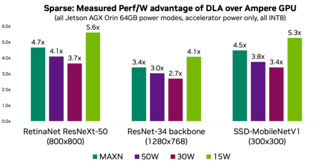
If power is one of your key KPIs, then you should consider DLA to take advantage of its power efficiency. DLA performance per watt is on average 3–5x more compared to the GPU, depending on the power mode and the workload. The following charts show performance per watt for three models representing common use cases.
Figure 1. DLA power efficiency
Figure 2. Structured Sparsity and performance per watt advantage
Put differently, without DLA’s power efficiency, it would not be possible to achieve up to 275 peak DL TOPs on NVIDIA Orin at a given platform power budget. For more information and measurements for more models, see the DLA-SW GitHub repo.
Here are some case studies within NVIDIA on how we used the AI compute offered by DLA: Automotive and Robotics
Case study: Automotive
NVIDIA DRIVE AV is the end-to-end autonomous driving solution stack for automotive OEMs to add autonomous driving and mapping features to their automotive product portfolio. It includes perception, mapping, and planning layers, as well as diverse DNNs trained on high-quality, real-world driving data.
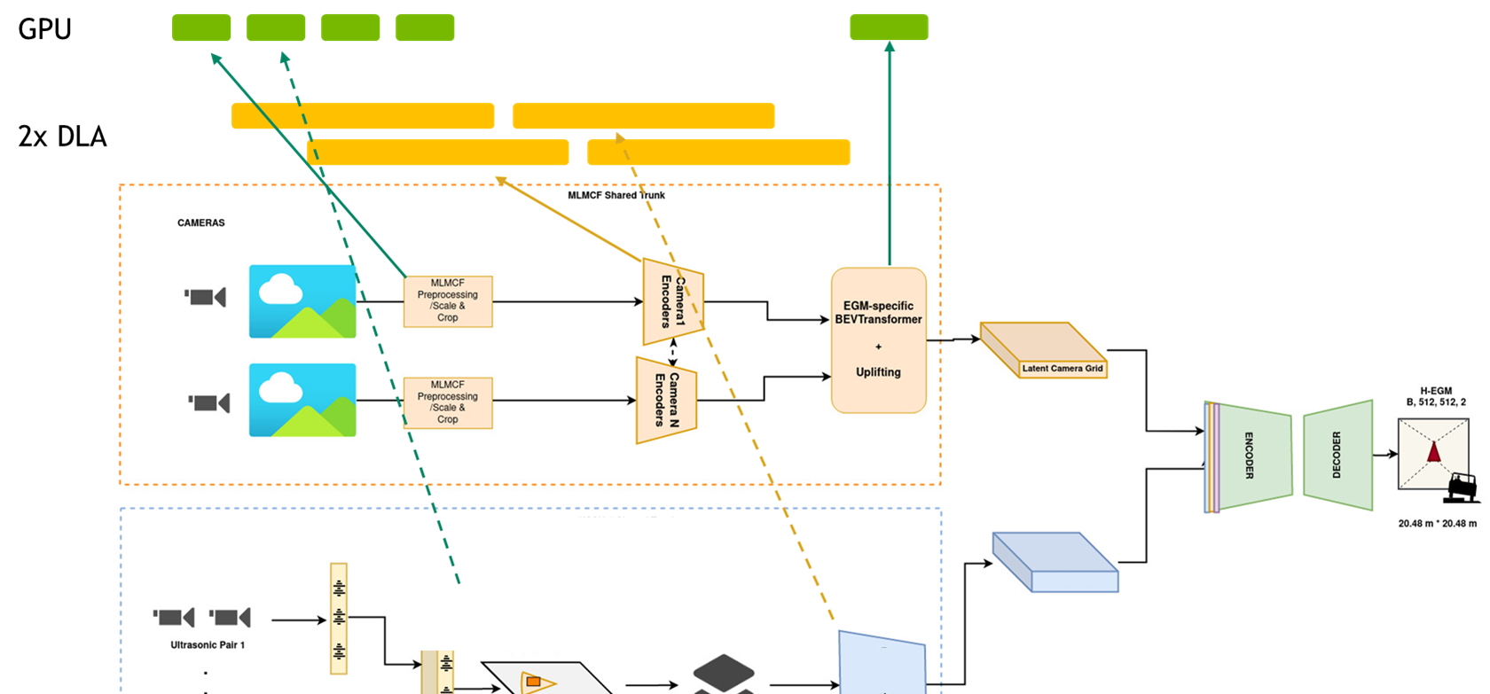
Engineers from the NVIDIA DRIVE AV team work on designing and optimizing the perception, mapping, and planning pipelines by leveraging the entire NVIDIA Orin SoC platform. Given the large number of neural networks and other non-DNN tasks to process in the self-driving stack, they rely on DLA as the dedicated inference engine on the NVIDIA Orin SoC, to run DNN tasks. This is critical because the GPU compute is reserved to process non-DNN tasks. Without DLA compute, the team would not meet their KPIs.
For instance, for the perception pipeline, they have inputs from eight different camera sensors and the latency of the entire pipeline must be lower than a certain threshold. The perception stack is DNN-heavy and accounts for more than 60% of all the compute.
To meet these KPIs, parallel pipeline tasks are mapped to GPU and DLA, where almost all the DNNs are running on DLAs and non-DNN tasks on the GPU to achieve the overall pipeline latency target. The outputs are then consumed sequentially or in parallel by other DNNs in other pipelines like mapping and planning. You may view the pipelines as a giant graph with tasks running in parallel on GPU and DLA. Using DLA, the team reduced their latency 2.5x.
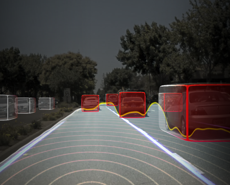
Figure 4. Object detection as part of the perception stack
“Leveraging the entire SoC, especially the dedicated deep learning inference engine in DLA, is enabling us to add significant functionality to our software stack while still meeting latency requirements and KPI targets. This is only possible with DLA,” said Abhishek Bajpayee, engineering manager of the Autonomous Driving team at NVIDIA.
Case study: Robotics
NVIDIA Isaac is a powerful, end-to-end platform for the development, simulation, and deployment of AI-enabled robots used by robotics developers. For mobile robots in particular, the available DL compute, deterministic latencies, and battery endurance are important factors. This is why mapping DL inference to DLA is important.
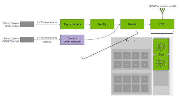
A team of engineers from the NVIDIA Isaac team have developed a library for proximity segmentation using DNNs. Proximity segmentation can be used to determine whether an obstacle is within a proximity field and to avoid collisions with obstacles during navigation. They implemented the BI3D network on DLA that performs binary depth classification from a stereo camera.
Figure 5. Proximity segmentation pipeline
Figure 5. Proximity segmentation pipeline NEEDS ALT TEXT A key KPI is ensuring real-time 30-fps detection from a stereo camera input. The NVIDIA Isaac team distributes the tasks across the SoC and uses DLA for the DNNs, while providing functional safety diversity in hardware and software from what is run on the GPU. For more information, see NVIDIA Isaac ROS Proximity Segmentation.
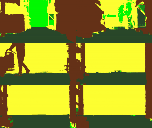
Figure 6. Proximity segmentation on a stereo input using BI3D.
“We use TensorRT on DLA for DNN inference to provide hardware diversity from the GPU improving fault tolerance while offloading the GPU for other tasks. DLA delivers ~46 fps on Jetson AGX Orin for BI3D, which consists of three DNNs, providing low 30 ms of latency for our robotics applications,” said Gordon Grigor, vice president of Robotics Platform Software at NVIDIA.
NVIDIA DeepStream for DLA
The quickest way to explore DLA is through the NVIDIA DeepStream SDK, a complete streaming analytics toolkit.
If you are a vision AI developer building AI-powered applications to analyze video and sensor data, the DeepStream SDK enables you to build optimal end-to-end pipelines. For cloud or edge use cases such as retail analytics, parking management, managing logistics, optical inspection, robotics, and sports analytics, DeepStream enables the use of the entire SoC and specifically DLA with little effort.
Replit aims to empower the next billion software creators. In this week’s episode of NVIDIA’s AI Podcast, host Noah Kraviz dives into a conversation with Replit CEO Amjad Masad. Read article >
Editor’s note: This post is part of Into the Omniverse, a series focused on how artists, developers and enterprises can transform their workflows using the latest advances in OpenUSD and NVIDIA Omniverse. Whether animating a single 3D character or generating a group of them for industrial digitalization, creators and developers who use the popular Reallusion Read article >
The start of a new school year is an ideal time for students to upgrade their content creation, gaming and educational capabilities by picking up an NVIDIA Studio laptop, powered by GeForce RTX 40 Series graphics cards. Read article >
When it comes to preserving profit margins, data scientists for vehicle and parts manufacturers are sitting in the driver’s seat. Viaduct, which develops models for time-series inference, is helping enterprises harvest failure insights from the data captured on today’s connected cars. Read article >
Optical Character Detection (OCD) and Optical Character Recognition (OCR) are computer vision techniques used to extract text from images. Use cases vary across…
Optical Character Detection (OCD) and Optical Character Recognition (OCR) are computer vision techniques used to extract text from images. Use cases vary across industries and include extracting data from scanned documents or forms with handwritten texts, automatically recognizing license plates, sorting boxes or objects in a fulfillment center based on serial numbers, identifying components for inspection on assembly lines based on part numbers, and more.
OCR is used in many industries, including financial services, healthcare, logistics, industrial inspection, and smart cities. OCR improves productivity and increases operational efficiency for businesses by automating manual tasks.
To be effective, OCR must achieve or exceed human-level accuracy. It is inherently complicated due to the unique use cases it works across. For example, when OCR is analyzing text, the text can vary in font, size, color, shape, and orientation, and can be handwritten or have other noise like partial occlusion. Fine-tuning the model on the test environment becomes extremely important to maintain high accuracy and reduce error rate.
NVIDIA TAO Toolkit is a low-code AI toolkit that can help developers customize and optimize models for many vision AI applications. NVIDIA introduced new models and features for automating character detection and recognition in TAO 5.0. These models and features will accelerate the creation of custom OCR solutions. For more details, see Access the Latest in Vision AI Model Development Workflows with NVIDIA TAO Toolkit 5.0.
This post is part of a series on using NVIDIA TAO and pretrained models to create and deploy custom AI models to accurately detect and recognize handwritten texts. This part explains the training and fine-tuning of character detection and recognition models using TAO. Part 2 walks you through the steps to deploy the model using NVIDIA Triton. The steps presented can be used with any other OCR tasks.
NVIDIA TAO OCD/OCR workflow
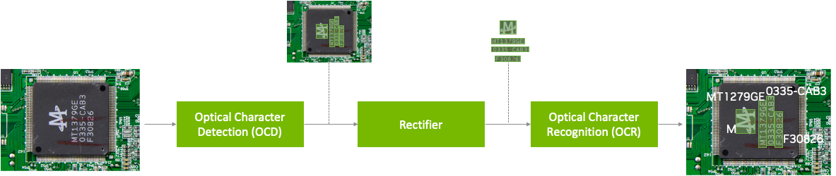
Figure 1. Character recognition pipeline with OCDNet and OCRNet
A pretrained model has been trained on large datasets and can be further fine-tuned with additional data to accomplish a specific task. The Optical Character Detection Network (OCDNet) is a TAO pretrained model that detects text in images with complex backgrounds. It uses a process called differentiable binarization to help accurately locate text of various shapes, sizes, and fonts. The result is a bounding box with the detected text.
A text rectifier is middleware that serves as a bridge between character detection and character recognition during the inference phase. Its primary function is to improve the accuracy of recognizing characters on texts that are at extreme angles. To achieve this, the text rectifier takes the vertices of polygons that cover the text area and the original images as inputs.
The Optical Character Recognition Network (OCRNet) is another TAO pretrained model that can be used to recognize the characters of text that reside in the detected bounding box regions. This model takes the image as network input and produces a sequence of characters as output.
Prerequisites
To follow along with the tutorial, you will need the following:
NVIDIA TAO Toolkit 5.0 (Installation instructions are included in the Jupyter notebooks). For a complete set of dependencies and prerequisites, see the TAO Toolkit Quick Start Guide.
Download the dataset
This tutorial fine-tunes the OCD and OCR model to detect and recognize handwritten letters. It works with the IAM Handwriting Database, a large dataset containing various handwritten English text documents. These text samples will be used to train and test handwritten text recognizers for the OCD and OCR models.
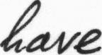
Figure 2. Handwritten word from the IAM dataset
To gain access to this dataset, register your email address on the IAM registration page.
Once registered, download the following datasets from the downloads page:
data/ascii.tgz
data/formsA-D.tgz
data/formsE-H.tgz
data/formsI-Z.tgz
The following section explores various aspects of the Jupyter notebook to delve deeper into the fine-tuning process of OCDNet and OCRNet for the purpose of detecting and recognizing handwritten characters.
Note that this dataset may be used for noncommercial research purposes only. For more details, review the terms of use on the IAM Handwriting Database.
Run the notebook
The OCDR Jupyter notebook showcases how to fine-tune the OCD and OCR models to the IAM handwritten dataset. It also shows how to run inference on the trained models and perform deployment.
Set up environment variables
Set up the following environment variables in the Jupyter notebook to match your current directory, then execute:
%env LOCAL_PROJECT_DIR=home//ocdr_notebook
%env NOTEBOOK_DIR=home//ocdr_notebook

# Set this path if you don't run the notebook from the samples directory.
%env NOTEBOOK_ROOT=home//ocdr_notebook
The following folders will be generated:
HOST_DATA_DIR contains the train/test split data for model training.
HOST_SPECS_DIR houses the specification files that contain the hyperparameters used by TAO to perform training, inference, evaluation, and model deployment.
HOST_RESULTS_DIR contains the results of the fine-tuned OCD and OCR models.
PRE_DATA_DIR is where the downloaded handwritten dataset files will be located. This path will be called to preprocess the data for OCD/OCR model training.
TAO Launcher uses Docker containers when running tasks. For data and results to be visible to Docker, map the location of our local folders to the Docker container using the ~/.tao_mounts.json file. Run the cell in the Jupyter notebook to generate the ~/.tao_mounts.json file.
The environment is now ready for use with the TAO Launcher. The next steps will prepare the handwritten dataset to be in the correct format for TAO OCD model training.
Prepare the dataset for OCD and OCR
Preprocess the IAM handwritten dataset to match the TAO image format following the steps below. Note that in the folder structure for OCD and OCR model training in TAO, /img houses the handwritten image data, and /gt contains ground truth labels of the characters found in each image.
Begin by moving the four downloaded .tgz files to the location of your $PRE_DATA_DIR directory. If you are following the same steps as above, the .tgz files will be placed in /data/iamdata.
Extract the images and ground truth labels from these files. The subsequent cells will extract the image files and move them to the proper folder format when run.
!tar -xf $PRE_DATA_DIR/ascii.tgz --directory $PRE_DATA_DIR/ words.txt

# Create directories to hold the image data and ground truth files.
!mkdir -p $PRE_DATA_DIR/train/img
!mkdir -p $PRE_DATA_DIR/test/img
!mkdir -p $PRE_DATA_DIR/train/gt
!mkdir -p $PRE_DATA_DIR/test/gt
# Unpack the images, let's use the first two groups of images for training, and the last for validation.

!tar -xzf $PRE_DATA_DIR/formsA-D.tgz --directory $PRE_DATA_DIR/train/img
!tar -xzf $PRE_DATA_DIR/formsE-H.tgz --directory $PRE_DATA_DIR/train/img
!tar -xzf $PRE_DATA_DIR/formsI-Z.tgz --directory $PRE_DATA_DIR/test/img
The data is now organized correctly. However, the ground truth label used by IAM dataset is currently in the following format:
a01-000u-00-00 ok 154 1 408 768 27 51 AT A


#     a01-000u-00-00  -> word id for line 00 in form a01-000u
#     ok              -> result of word segmentation
#                            ok: word was correctly
#                            er: segmentation of word can be bad
#
#     154            -> graylevel to binarize the line containing this word
#     1               -> number of components for this word
#     408 768 27 51   -> bounding box around this word in x,y,w,h format
#     AT            -> the grammatical tag for this word, see the
#                        file tagset.txt for an explanation
#     A               -> the transcription for this word
The words.txt file looks like this:
  		0				1
0	a01-000u-00-00	ok 154 408 768 27 51 AT A
1	a01-000u-00-01	ok 154 507 766 213 48 NN MOVE
2	a01-000u-00-02	ok 154 796 764 70 50 TO to
...
Currently, words.txt uses a four-point coordinate system for drawing a bounding box around the word in an image. TAO requires the use of an eight-point coordinate system to draw a bounding box around detected text.
To convert the data to the eight-point coordinate system, use the extract_columns and process_text_file functions provided in section 2.1 of the notebook. words.txt will be transformed into the following DataFrame and will be ready for fine-tuning on an OCDNet model.
filename	   x	 y	x2	y2	x3	y3	x4	y4	word
0	gt_a01-000u.txt	  408	768	435	768	435	819	408	819	A
1	gt_a01-000u.txt	  507	766	720	766	720	814	507	814	MOVE
2	gt_a01-000u.txt	  796	764	866	764	866	814	796	814	to
...
To prepare the dataset for OCRNet, the raw image data and labels must be converted to LMDB format, which converts the images and labels into a key-value memory database.
# Convert the raw train and test dataset to lmdb
print("Converting the training set to LMDB.")
!tao model ocrnet dataset_convert -e $SPECS_DIR/ocr/experiment.yaml
                        	dataset_convert.input_img_dir=$DATA_DIR/train/processed
                        	dataset_convert.gt_file=$DATA_DIR/train/gt.txt
                        	dataset_convert.results_dir=$DATA_DIR/train/lmdb

# Convert the raw test dataset to lmdb
print("Converting the testing set to LMDB.")
!tao model ocrnet dataset_convert -e $SPECS_DIR/ocr/experiment.yaml
                        	dataset_convert.input_img_dir=$DATA_DIR/test/processed
                        	dataset_convert.gt_file=$DATA_DIR/test/gt.txt
                        	dataset_convert.results_dir=$DATA_DIR/test/lmdb
The data is now processed and ready to be fine-tuned on the OCDNet and OCRNet pretrained models.
Create a custom character detection (OCD) model
The NGC CLI will be used to download the pretrained OCDNet model. For more information, visit NGC and click on Setup in the navigation bar.
Download the OCDNet pretrained model
!mkdir -p $HOST_RESULTS_DIR/pretrained_ocdnet/

# Pulls pretrained models from NGC
!ngc registry model download-version nvidia/tao/ocdnet:trainable_resnet18_v1.0 --dest $HOST_RESULTS_DIR/pretrained_ocdnet/
You can check that the model has been downloaded to /pretrained_ocdnet/ using the following call:
print("Check that model is downloaded into dir.")
!ls -l $HOST_RESULTS_DIR/pretrained_ocdnet/ocdnet_vtrainable_resnet18_v1.0
OCD training specification
In the specs folder, you can find different files related to how you want to train, evaluate, infer, and export data for both models. For training OCDNet, you will use the train.yaml file in the specs/ocd folder. You can experiment with changing different hyperparameters, such as number of epochs, in this spec file.
Below is a code example of some of the configs that you can experiment with:
Now that the specification files are configured, provide the paths to the spec file, the pretrained model, and the results:
#Train using TAO Launcher
#print("Run training with ngc pretrained model.")
!tao model ocdnet train
      	-e $SPECS_DIR/train.yaml
      	-r $RESULTS_DIR/train
      	model.pretrained_model_path=$DATA_DIR/ocdnet_deformable_resnet18.pth
Training output will resemble the following. Note that this step could take some time, depending on the number of epochs specified in train.yaml.
LOCAL_RANK: 0 - CUDA_VISIBLE_DEVICES: [0]
  | Name  | Type  | Params
--------------------------------
0 | model | Model | 12.8 M
--------------------------------
12.8 M    Trainable params
0         Non-trainable params
12.8 M    Total params
51.106    Total estimated model params size (MB)
Training: 0it [00:00, ?it/s]Starting Training Loop.
Epoch 0: 100%|█████████| 751/751 [19:57
Evaluate the model
Next, evaluate the OCDNet model trained on the IAM dataset.
# Evaluate on model
!tao model ocdnet evaluate
        	-e $SPECS_DIR/evaluate.yaml
        	evaluate.checkpoint=$RESULTS_DIR/train/model_best.pth
Evaluation output will look like the following:
test model: 100%|██████████████████████████████| 488/488 [06:44
OCD inference
The inference tool produces annotated image outputs and .txt files that contain prediction information. Run the inference tool below to generate inferences on OCDNet models and visualize the results for detected text.
# Run inference using TAO
!tao model ocdnet inference
       	-e $SPECS_DIR/ocd/inference.yaml
       	inference.checkpoint=$RESULTS_DIR/ocd/train/model_best.pth
       	inference.input_folder=$DATA_DIR/test/img
       	inference.results_dir=$RESULTS_DIR/ocd/inference
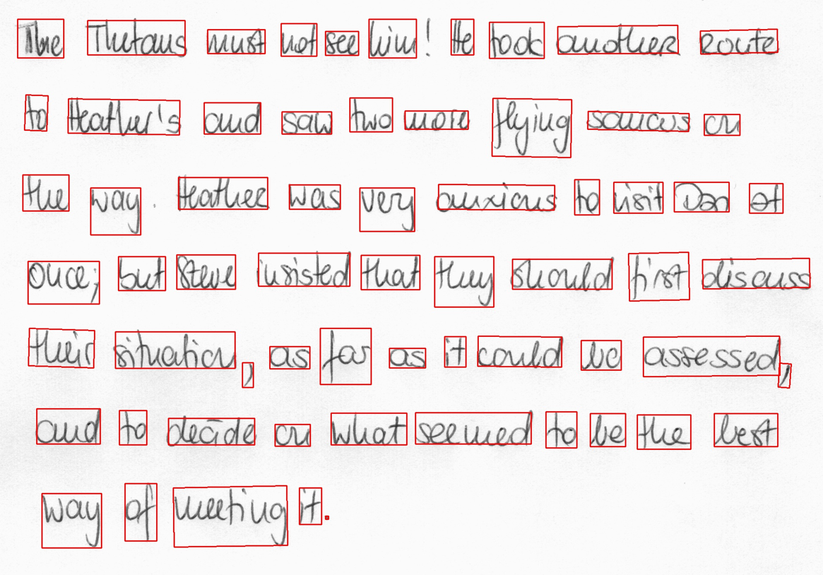
Figure 3 shows the OCDNet inference on a test sample image.
Figure 3. Output from OCDNet inference
Export the OCD model for deployment
The last step is to export the OCD model to ONNX format for deployment.
!tao model ocdnet export
       	-e $SPECS_DIR/export.yaml
       	export.checkpoint=$RESULTS_DIR/train/model_best.pth
       	export.onnx_file=$RESULTS_DIR/export/model_best.onnx
Create a custom character recognition (OCR) model
Now that you have the trained OCDNet model to detect and apply bounding boxes to areas of handwritten text, use TAO to fine-tune the OCRNet model to recognize and classify the detected letters.
Download the OCRNet pretrained model
Continuing in the Jupyter notebook, the OCRNet pretrained model will be pulled from NGC CLI.
!mkdir -p $HOST_RESULTS_DIR/pretrained_ocrnet/

# Pull pretrained model from NGC
!ngc registry model download-version nvidia/tao/ocrnet:trainable_v1.0 --dest $HOST_RESULTS_DIR/pretrained_ocrnet
OCR training specification
OCRNet will use the experiment.yaml spec file to perform training. You can change training hyperparameters such as batch size, number of epochs, and learning rate shown below:
Train the OCRNet model on the dataset. You can also configure spec parameters like the number of epochs or learning rate within the train command, shown below.
You can evaluate the OCRNet model based on the accuracy of its character recognition. Recognition accuracy simply means a percentage of all the characters in a text area that were recognized correctly.
!tao model ocrnet evaluate -e $SPECS_DIR/ocr/experiment.yaml
             	evaluate.results_dir=$RESULTS_DIR/ocr/evaluate
             	evaluate.checkpoint=$RESULTS_DIR/ocr/train/best_accuracy.pth
             	evaluate.test_dataset_dir=$DATA_DIR/test/lmdb
             	dataset.character_list_file=$DATA_DIR/train/character_list.txt
Evaluation
The output should appear similar to the following:
data directory:	/data/iamdata/test/lmdb	 num samples: 37109
Accuracy: 77.8%
OCR inference
Inference on OCR will produce a sequence output of recognized characters from the bounding boxes, shown below.
!tao model ocrnet inference -e $SPECS_DIR/ocr/experiment.yaml
inference.results_dir=$RESULTS_DIR/ocr/inference
inference.checkpoint=$RESULTS_DIR/ocr/train/best_accuracy.pth
inference.inference_dataset_dir=$DATA_DIR/test/processed
dataset.character_list_file=$DATA_DIR/train/character_list.txt
Finally, export the OCD Model to ONNX format for deployment.
!tao model ocrnet export -e $SPECS_DIR/ocr/experiment.yaml
             	export.results_dir=$RESULTS_DIR/ocr/export
             	export.checkpoint=$RESULTS_DIR/ocr/train/best_accuracy.pth
             	export.onnx_file=$RESULTS_DIR/ocr/export/ocrnet.onnx
             	dataset.character_list_file=$DATA_DIR/train/character_list.txt
Results
Table 1 highlights the accuracy and performance of the two models featured in this post. The character detection model is fine-tuned on the ICDAR pretrained OCDNet model and character recognition model is fine-tuned on the Uber-text OCRNet pretrained model. ICDAR and Uber-text are publicly available datasets that we used to pretrain the OCDNet and OCRNet models, respectively. Both models are available on NGC.
Table 1. Performance and accuracy data for OCDNet and OCRNet
Summary
This post explains the end-to-end workflow for creating custom character detection and recognition models in NVIDIA TAO. You can start with a pretrained model for character detection (OCDNet) and character recognition (OCRNet) from NGC. Then fine-tune it on your custom dataset using TAO and export the model for inference.
Continue reading Part 2 for a step-by-step walkthrough on deploying this model into production using NVIDIA Triton.

 Demand for real-time insights and autonomous decision-making is growing in various industries. To meet this demand, we need scalable edge-solution platforms…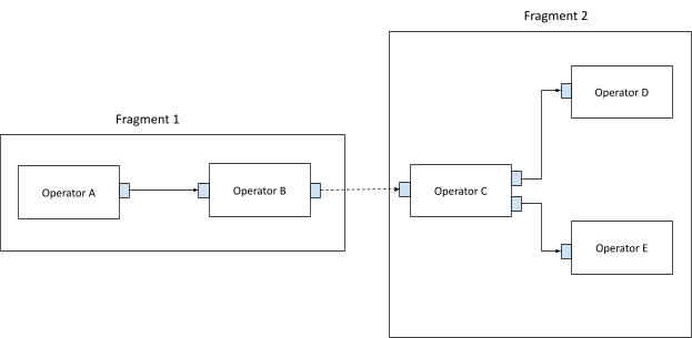
 Deep neural networks (DNNs) are the go-to model for learning functions from data, such as image classifiers or language models. In recent years, deep models…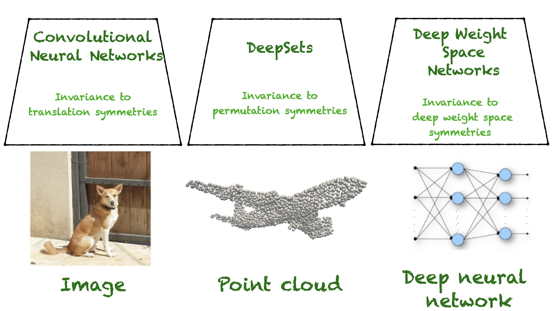

![[W_m, b_l]_{ m in [M],lin[M]}](https://s0.wp.com/latex.php?latex=%5BW_m%2C+b_l%5D_%7B+m+%5Cin+%5BM%5D%2Cl%5Cin%5BM%5D%7D&bg=transparent&fg=000&s=0&c=20201002) . Importantly, in this setup, the weight space is the input space to the (soon-to-be-defined) neural networks.
. Importantly, in this setup, the weight space is the input space to the (soon-to-be-defined) neural networks.

 and
and  cancel each other (assuming an elementwise activation function like ReLU).
 represents permutation matrices. This observation was made more than 30 years ago by Hecht-Nielsen in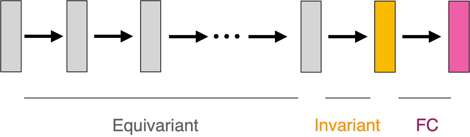
 as a block matrix whose (i,j)-th block is a linear equivariant layer between
  and
and 
 . This block structure is illustrated in Figure 4.
 ? Our paper lists all the possible cases and shows that some of these layers were already characterized in previous work. For example,
  for internal layers was characterized in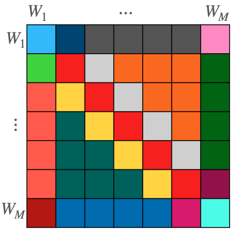
 NVIDIA Jetson Orin is the best-in-class embedded AI platform. The Jetson Orin SoC module has the NVIDIA Ampere architecture GPU at its core but there is a lot…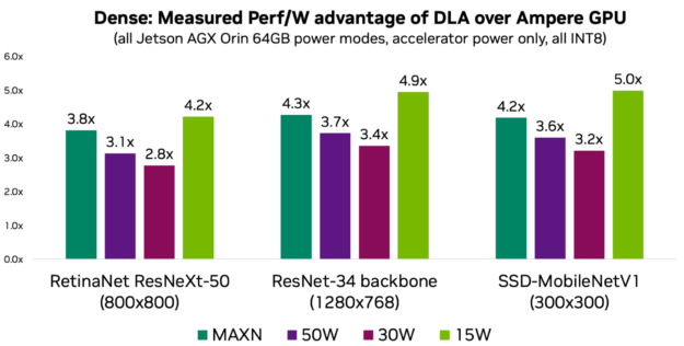
 On Aug. 29, learn how to create efficient AI models with NVIDIA TAO Toolkit on STM32 MCUs.
 Optical Character Detection (OCD) and Optical Character Recognition (OCR) are computer vision techniques used to extract text from images. Use cases vary across…