This week In the NVIDIA Studio, we’re launching the April NVIDIA Studio Driver with optimizations for the most popular 3D apps, including Unreal Engine 5, Cinema4D and Chaos Vantage. The driver also supports new NVIDIA Omniverse Connectors from Blender and Redshift.
Take a deep dive into the integrated cloud-ready infrastructure solution from Red Hat and NVIDIA
The IT world is moving to cloud, and cloud is built on containers managed with Kubernetes. We believe the next logical step is to accelerate this infrastructure with data processing units (DPUs) for greater performance, efficiency, and security.
Red Hat and NVIDIA are building an integrated cloud-ready infrastructure solution with the management and automation of Red Hat OpenShift combined with the acceleration, workload isolation, and security capabilities of NVIDIA BlueField DPUs.
Benefits of Red Hat OpenShift
Many popular cloud infrastructure projects use containers managed by Kubernetes. However, implementing Kubernetes can be a heavy lift, especially for organizations that cannot devote dedicated staff to becoming Kubernetes experts.
Red Hat OpenShift provides a powerful set of capabilities for managing Kubernetes containers as well as application deployment, updates, and lifecycle management. OpenShift includes automation and security tools, as well as a supported open-source model to make cloud infrastructure more affordable, reliable, and scalable.
According to a 2021 Red Hat survey, Kubernetes is used for over 85% of container orchestration projects, and Red Hat OpenShift is the most popular choice for hybrid and multicloud Kubernetes deployments. OpenShift is the industry’s leading enterprise Kubernetes platform, used by more than 50% of commercial banks, telecommunications companies, and airlines on the Fortune 500.
It is clear that most enterprises want a supported Kubernetes model, and Red Hat OpenShift is one of the most popular choices.
How a DPU works
A DPU offloads, accelerates, and isolates infrastructure workloads from the server’s CPU. For example, the BlueField DPU can offload networking, network virtualization, data encryption, and time synchronization tasks from the CPU and run them on purpose-built silicon.
Other infrastructure software, such as remote management, firewall agents, network control plane, and storage virtualization, can run on BlueField’s Arm processor cores. Doing so frees up the server’s CPU cores that can instead run applications and tenant workloads.
This functionality also isolates infrastructure and security workloads in a separate domain. The result is a set of servers that run more applications with faster networking, increasing the efficiency and security of the data center.
In a typical cloud infrastructure, the network traffic traverses both physical servers and containers running on these servers. This requires a packet switching solution within each server, and to gain maximum efficiency, the application containers need a way to talk to the accelerated networking offloads of the DPU.
The traditional way is to go through Kubernetes and Open Virtual Network (OVN) to access the Open Virtual Switch (Open vSwitch or OVS). OVN provides network abstraction and the default deployment strategy is to run both OVN and OVS on the host server’s CPU.
However, this method consumes a significant number of CPU cores as the network speeds increase beyond 10 Gbps. A solution is needed for Kubernetes to run the OVN and OVS functionality on the DPU so that all the packet switching, header rewrites, encapsulation/decapsulation, and packet filtering can be done on networking hardware instead of in software on the CPU.
Increasing networking integration between Red Hat and NVIDIA
Red Hat and NVIDIA have collaborated to integrate the management power of OpenShift with the acceleration capabilities of the DPU.
The first stage of integration started in 2018 with Red Hat Enterprise Linux offloading network traffic to the NVIDIA ConnectX SmartNIC. The networking data plane–using OVS or DPDK–was running on the SmartNIC ASIC but the networking control plane was still running entirely in software on the X86 CPU.
Figure 1. OpenStack SDN controller, running on Red Hat Enterprise Linux, offloads the networking data plane to the NVIDIA ConnectX SmartNIC through OVS while the control plane runs on the X86 CPU.
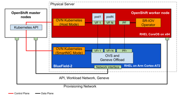
In this solution, the networking data plane with overlay offload (OVS and Geneve Offload) and the networking control plane (in the OVN Kubernetes pod) were running on the DPU with Red Hat Enterprise Linux. The major OpenShift components, including Red Hat Enterprise Linux CoreOS remained on the x86 CPU.
Figure 2. Red Hat OpenShift, running on Red Hat Enterprise Linux CoreOS, offloads both the networking data plane and control plane to the BlueField-2 DPU, via OVN and OVS. The DPU is running Red Hat Enterprise Linux on its Arm cores.
In the deployment scenario in Figure 2, the BlueField-2 does the heavy lifting in the following areas:
The host CPU and container see only simple unencapsulated, unencrypted packets and the CPU does not need to perform any of these tasks because they are offloaded to the DPU. This level of offload reduced CPU utilization by 70%, freeing up substantial CPU power on each server to run additional business/tenant workloads.
Running OpenShift on the DPU
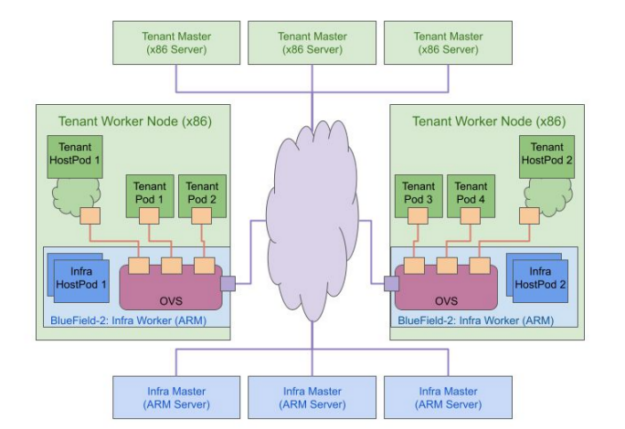
As presented at GTC 2022, Red Hat and NVIDIA have taken the next step, moving OpenShift, including Red Hat Enterprise Linux CoreOS, to run on the Arm cores of the BlueField DPU for the Red Hat OpenShift two cluster design that includes separate tenant and infrastructure clusters.
Red Hat Enterprise Linux CoreOS is the supported operating system for the OpenShift control plane, or master and worker nodes. This is the portion of OpenShift that performs scheduling, maintenance, upgrades, and cluster automation. It includes container management tools and security hardening to make it more resistant to hackers, and it now runs on both the host x86 CPU and on the DPU Arm cores.
BlueField DPUs running OpenShift OVS and OVN containers and Red Hat Enterprise Linux CoreOS on the various host servers form an infrastructure worker cluster. Meanwhile, OpenShift running on the x86 CPUs manages the tenant pods and clusters.
Offloading the OpenShift infrastructure cluster software to run on the BlueField Arm cores instead of on the host x86 cores provides additional x86 CPU savings, higher performance, and stronger security isolation.
Figure 3. Starting with Red Hat OpenShift 4.10, you can run OpenShift on both the x86 CPUs to manage the tenants and on the BlueField DPU Arm cores to manage the cluster infrastructure.
The cloud-native, software-defined networking is a good example of a BlueField DPU use case where OVN and OVS are running on and offloaded by the BlueField DPU in an OpenShift environment. Many other infrastructure services, such as network encryption, firewall agents, virtual routers, telemetry agents, and so on, can also be run on the DPU for an even greater benefit.
Significant cost savings benefits from OpenShift Offload on DPU
To understand the impact of the DPU offloads on reducing the data center costs, NVIDIA and Red Hat put together a TCO model for a mid-sized data center with 51K servers. We considered this data center to be supporting 1M applications, each application needing 10K packets per second (PPS) of switching performance.
The server with no DPU running the virtual switching entirely in software achieved only 350k PPS.
The server with a DPU that offloads OVN and OVS to the DPU achieved 54x times higher performance of 18.7 million PPS per server.
Offloading virtual switching to the DPU also saved eight CPU cores per server. Based on this testing, the TCO model yielded amazing savings of $68.5M of CapEx. These savings are recognized by requiring 10K fewer DPU-enhanced servers due to much higher networking performance and CPU core savings per server.
We see power savings due to the smaller server footprint, which ultimately results in a better TCO model with the DPU-based servers. These TCO savings will get even better as we offload additional functions such as load balancers, firewalls, encryption, web servers, and so on to the DPUs, ultimately achieving amazing efficiency for cloud-ready data centers.
Solution roadmap and deploying OpenShift on BlueField
The two-cluster OpenShift architecture running OpenShift on BlueField is now available as a developer preview or early trial in OpenShift 4.10, and is expected to become generally available in 2022.
But the NVIDIA and Red Hat teams aren’t stopping here. We are planning to test the offloading of network traffic encryption/decryption as that is a CPU-intensive task.
BlueField-2 DPU can offload IPsec encryption/decryption at up to 100 Gbps and TLS encryption/decryption at up to 200 Gbps.
BlueField-3 is expected to support IPSec, TLS and MACsec at even higher speeds.
Implementation of line-rate encryption offload from OpenShift to the DPU will improve data security for tenants and help you move closer to a zero-trust security stance.
Other potential integrations with the DPU include more sophisticated software-defined networking offloads, running a firewall agent on BlueField, precision time synchronization, video streaming with packet pacing, and using the DPU to collect telemetry data.
BlueField-2 DPUs are available now from NVIDIA and the BlueField-3 DPU will start sampling later in 2022. In addition, BlueField DPUs will soon be available for testing in the NVIDIA LaunchPad cloud service.
If you would like to test or develop on Red Hat OpenShift running with the NVIDIA BlueField DPU, please indicate your interest.
Summary
If your organization seeks to embrace cloud-native computing in data centers, the combination of NVIDIA BlueField DPUs, Red Hat Enterprise Linux, and Red Hat OpenShift provides an efficient and innovative open, hybrid-cloud platform with new security features. This powerful platform delivers hardware acceleration capabilities to run critical software-defined networking, storage, and security functions.
Now more server resources can be allocated to run cloud-native workloads, as well as traditional business applications.
For more information, see the following resources:
I’m a newbee in the machine learning frameworks. When I’m learning machine learning frameworks such as TensorFlow, PyTorch, and MindSpore, I’m confused between accuracy and precision. What is the difference when we say to improve model accuracy and to improve model precision? Can you help me to figure it out? Thanks
I built a custom generator that outputs X data with shape (100,2,2048) belonging to Y 16 (16) classes to be passed to a GRU model for video classification.
100 is the sequence length, 2 is for 2 simultaneous camera views, each with 2048 features, extracted earlier with a feature extractor.
I need to pass this to GRU model, but it throws an error (Input 0 of layer “gru” incompatible with the layer: expected ndim=3, found ndim=4. Full shape received: (None,100,2,2048)
) when I set the input shape in the input layer to (100,2,2048).
Using just one camera view and setting the it to (100,2048) works.
What input shape do I need to set to accommodate the two cameras?
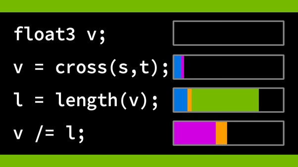
This is a deep dive into the Shader Profiler feature of NVIDIA Nsight Graphics. The Shader Profiler allows you to find hotspots in your shaders and why they’re hot.
A less well-known but cool feature of NVIDIA Nsight Graphics is the Shader Profiler. This enables you to find hot spots in your shaders that can help you to direct optimization effort. It can give you insights into why performance is sometimes not what you might like.
In this post, we use the NVIDIA Nsight Graphics Trace Analysis tool to identify a potential limiter and then use the Shader Profiler to dig deeper to find and fix an issue.
Step 1: Start with GPU Trace Analysis tool
We always recommend starting with the Nsight Graphics GPU Trace tool rather than diving straight into the shader profiler. That way, you can understand what the performance limiters of any given DX12 or VK workload are. For example, there’s no point trying to fine-tune your shader if the real problem is that you have low GPU utilization because you have lots of tiny dispatches with barriers between them all.
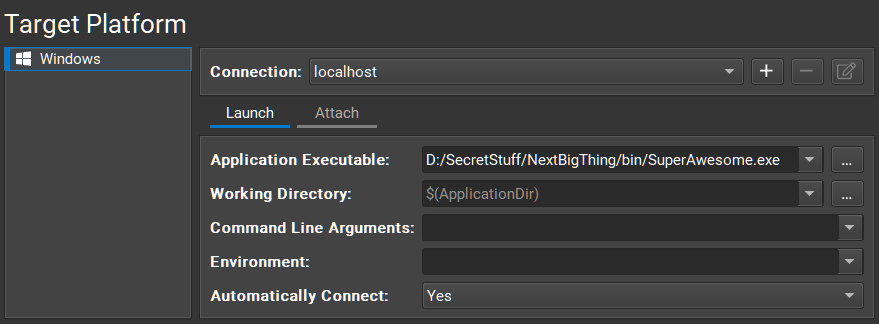
First, set up a connection to the app to be profiled. Choose Connect and fill in the required parameters for launching your game (Figure 1).
Figure 1. Connection settings
Select GPU Trace as the activity, with Metric Set configured to Advanced Mode Metrics. Using Advanced Mode Metrics requires a stable and consistent frame, because the analysis runs over several passes over several frames. If your application doesn’t meet these requirements, you can use the Nsight Graphics built-in C++ Capture tool to capture a frame of your application and create a new EXE that replays the same frame repeatedly.
Choose Launch GPU Trace to launch your application. When you reach a frame that you’d like to capture, choose Generate GPU Trace Capture or press F11.
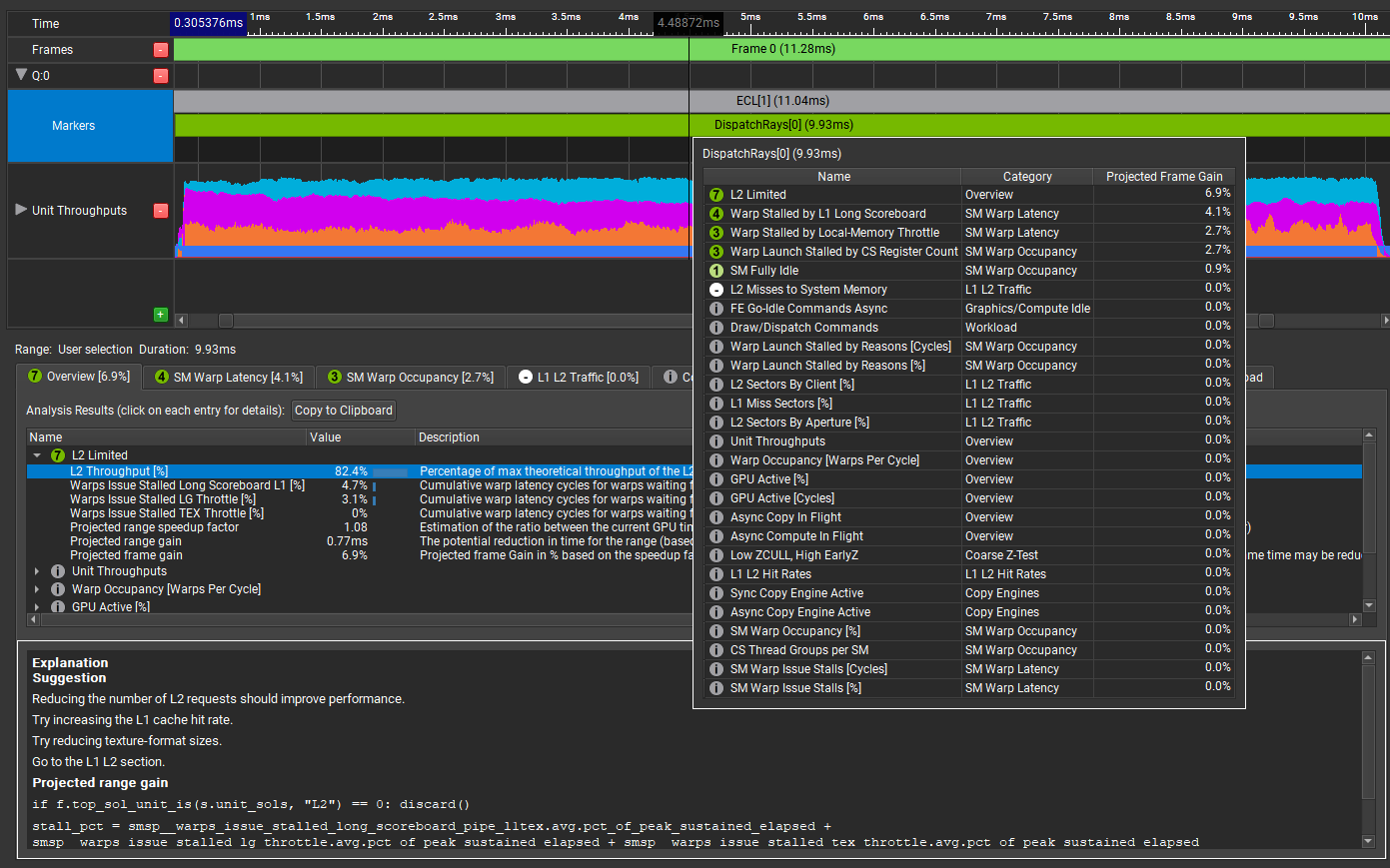
When the capture is complete, stop the application and open the trace. Choose Trace Analysis. In the Analysis panel of GPU Trace (Figure 2), double-click or hover over the marker for the range to analyze, in this case, DispatchRays[0]:
Figure 2. Trace Analysis results
The tooltip presents a compact view of all performance gain opportunities that the tool has detected in this GPU workload, sorted by their projected GPU frame-time gain. The workload has the following limiters:
L2 Limited: Being L2 limited might be indicative of a problem. With knowledge of the workload, it’s not necessarily something that you would expect.
Warp Stalled by L1 Long Scoreboard: This is a common reason for warps to be stalled, often due to texture fetches. If there is not enough work between a texture lookup being initiated and the result of the lookup being used, then the warp is stalled until the texture lookup is satisfied.
Warp Stalled by Local-Memory Throttle: Local memory is ‘thread local’. It’s memory that is local to each thread, as opposed to group-shared memory that is shared between all the threads in the thread group. It’s unusual for a shader to need any local memory, so this is interesting. And what does local-memory throttling mean? There’s more to learn here.
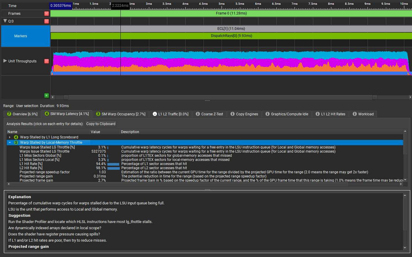
Choose SM Warp Latency and Warp Stalled by Local-Memory Throttle.
Figure 3. Trace Analysis explanation of Local Memory Throttle
The Explanation window gives a more meaningful description of the problem, with some helpful suggestions. It suggests launching the Shader Profiler to locate the specific HLSL instructions that have lg_throttle stalls.
Step 2: Switch to the Shader Profiler
Before you use the Shader Profiler, it’s important to make sure that Nsight Graphics can get access to symbols for your shaders. The easiest way to achieve this is to make sure that the shaders are compiled with the /Zi option, and embed the symbols in the shader binary.
Sometimes it’s preferable to configure the compilation so that the symbols go into an external PDB file. In that case, be sure to specify the correct path under Tools, Options.
When Nsight Graphics can see the shader symbols, it can map locations in the shader back to the source code, which makes it far easier for you to tell what’s going on. If Nsight Graphics doesn’t have access to symbols, then you can only see the shader disassembly (for example, DXIL).
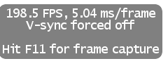
The Shader Profiler is part of the Frame Profiler. Connect to the application again but this time, choose Frame Profiler under Activity. When you choose Launch Frame Profiler, the application should launch with this HUD (Figure 4) on top of it.
Figure 4. Profiler overlay
Navigate to the part of the application to profile and press F11 to capture a frame for analysis. From here, choose Profile Shaders in Nsight Graphics. This runs a short sampling session, and then presents you with a summary view (Figure 5).
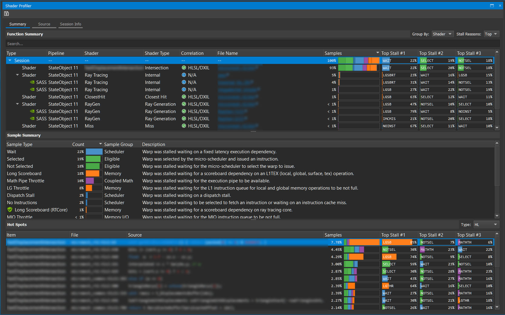
Figure 5. Shader Profiler summary view
Here’s a breakdown.
The Function Summary shows a list of the top shaders, in order of the number of samples that hit in those shaders. This is a good proxy for the shader latency and lets you concentrate on the shaders that can yield the biggest benefit from optimizing.
In the Correlation column, there are multiple green ticks, which are always good. In this case, it means that Nsight Graphics has been able to correlate the samples back to the source code.
To open up the shader view, select the first file name. On the left is the source code, and on the right is DXIL. For the purposes of this post, you don’t have to care about the DXIL, so change the view to just HLSL
It’s quite subtle, but there’s an important heat map of instruction samples on the far right, just to the right of the scroll bar. Remember, GPU Trace Analysis suggested that you should look for lg_throttle stalls. It said:
LSU is the unit that performs access to Local and Global memory. Run the Shader Profiler and locate which HLSL instructions have most lg_thottle stalls. Are dynamically indexed arrays declared in local scope? Does the shader have register pressure causing spills? If L1 and L2 hit rates are poor, then try to reduce misses.
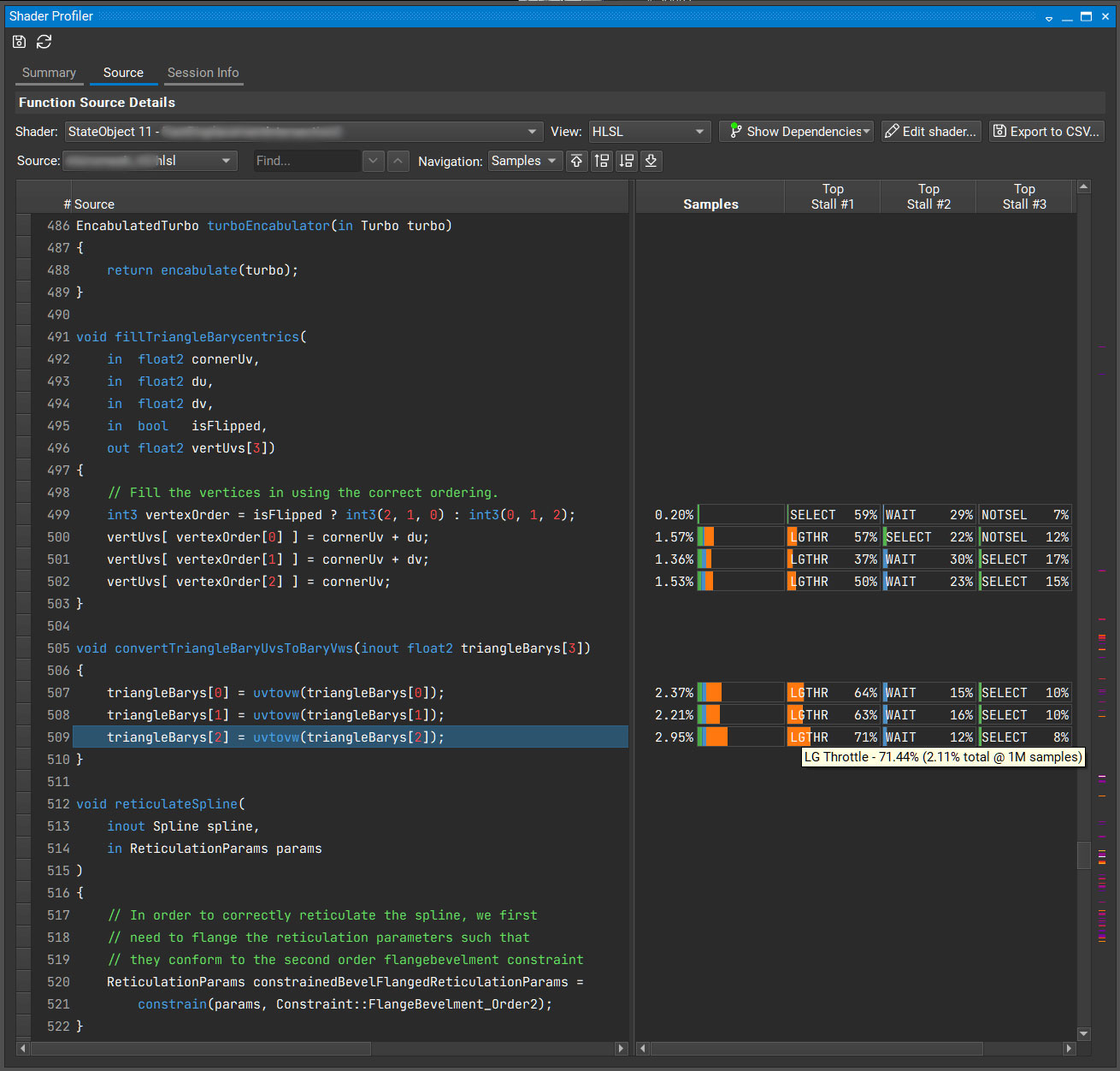
In the Shader Profiler, the samples that show as LGTHR are stalled due to lg_throttle reasons.
Figure 6. Shader Profiler source view with samples and stall reasons
“Are dynamically indexed arrays declared in local scope?”
Dynamically indexed arrays are indexed by a variable, where the value of the index is not known at compile time.
When this happens, the compiler often puts the array in local memory instead of it living in registers. Memory is slower than registers.
The following code example shows a dynamically indexed array.
The act of dynamically indexing this array makes the compiler move this array into memory. It affects this bit of code and all the bits of code that reference that array. That’s why convertTriangleBaryUvsToBaryVws is showing up as hot, too.
Can you do this without dynamic indexing? Yes, you can. Changing how the flip is done results in Figure 7.
Figure 7. Alternative code not using dynamic indexing
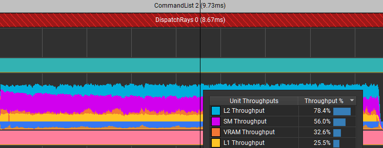
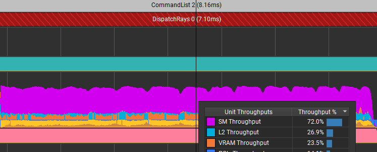
Those particular stalls are eliminated. It reduced the time for this dispatch from 8.67 ms down to 7.1 ms. Not only did it improve the efficiency of shader code, but it also massively reduced the limiter in L2 because of the reduced memory traffic.
Figure 8. Trace before optimization
Figure 9. Trace after optimization
Summary
NVIDIA Nsight Graphics is a powerful tool for analyzing your rendering workloads. This has been a quick walkthrough, just touching on some capabilities. We highly recommend using it.
Disclaimer
The tests and results in this post were true as of driver version 467.07. Driver and compiler development continues all the time. That means that optimization opportunities can change over time too.
Bit of a newbie to TF/the machine learning world. I’ve built/trained image classification & segmentation models before and have tinkered with TF recommenders before. My knowledge probably doesn’t go beyond the first few layers of the documentation/tutorials, though.
I’m wondering as to how I might accomplish something along these lines: I have approximately 20,000 images and I have manually placed a simple text watermark over the image to partially cover the subject of the image (the subject takes up 80% of the image and the watermark takes up approx 5% of the image), the watermark is small and subtle, only really noticeable if you zoom in. I have saved the coordinates for each watermark for each image file. I’m now looking to automate the placing of watermarks in a subtle position on the subject.
Could someone please link to some documentation/guides which would be appropriate for training a model to achieve this goal? I am assuming I need something along the lines of image classification but a lot of what I’m seeing is that it’s just for classifying what’s in an image/segmenting (drawing a box) around an object in the image rather than saying “given this image, this particular point on the subject in the image is relevant”.
When brainstorming a scene to best showcase the groundbreaking capabilities of the Omniverse platform, some NVIDIA artists turned to a cherished memory: enjoying ramen together in a mom-and-pop shop down a side street in Tokyo. Simmering pots of noodles, steaming dumplings, buzzing kitchen appliances, warm ambient lighting and glistening black ledger stools. These were all Read article >
I am a beginner in the machine learning field and while learning the tensorflow introductory I understood that tensor is just nothing but a generalized name for quantities that require multiple variables (features) for it’s description.
Then there is this line -> Matrix and Vectors are the tensors with different rank. Matrix is 2d tensor and vector is 1 d tensor.
A tensor is often thought of as a generalized matrix. That is, it could be a 1-D matrix (a vector is actually such a tensor)
I am coming from the CS background where I have learnt that 1D is array 2D is matrix and we used to take 1D array like std::vector<float> height_vector
So what is difference between arr[10] and arr[1][10] or arr[10][1] ?
A paper released today describes in the greatest detail to date the atmospheres on distant planets. Seeking the origins of what’s in and beyond the Milky Way, researchers surveyed 25 exoplanets, bodies that orbit stars far beyond our solar system. Specifically, they studied hot Jupiters, the largest and thus easiest to detect exoplanets, many sweltering Read article >

 Take a deep dive into the integrated cloud-ready infrastructure solution from Red Hat and NVIDIA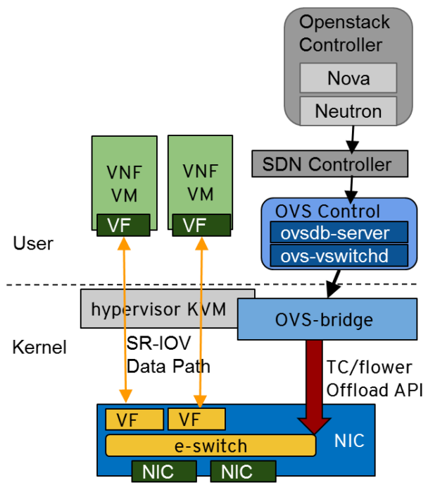



 This is a deep dive into the Shader Profiler feature of NVIDIA Nsight Graphics. The Shader Profiler allows you to find hotspots in your shaders and why they’re hot.