Categories
Misc

Scaling Quantum Circuit Simulation with NVIDIA cuTensorNet

Icon of NVIDIA green circle with an arrow pointing diagonally up right.We present benchmarks and usage of cuTensorNet, a cuQuantum library providing high-performance tensor network computations for quantum circuit simulation.
Icon of NVIDIA green circle with an arrow pointing diagonally up right.

Quantum computing aspires to deliver more powerful computation in faster time for problems that cannot currently be addressed with classical computing. NVIDIA recently announced the cuQuantum SDK, a high-performance library for accelerating the development of quantum information science. cuQuantum recently was used to break the world record for the MaxCut quantum algorithm simulation running on the DGX SuperPOD, with 8x more qubits than prior work.

The initial target application for cuQuantum is acceleration of quantum circuit simulations, and it consists of two major libraries: 

  • cuStateVec: Accelerates state vector simulations.
  • cuTensorNet: Accelerates tensor network simulations.

In this post, we provide an overview of both libraries, with a more detailed discussion of cuTensorNet.

Why use cuStateVec?

The cuStateVec library from the cuQuantum SDK provides a high-performance solution for state vector-based simulation through optimized GPU kernels for most use cases that arise in simulators. While the state vector method is great for running deep quantum circuits, simulations of quantum circuits with large numbers of qubits, which grow exponentially, are impossible to run even on today’s largest supercomputers. 

Why use cuTensorNet?

As an alternative, the tensor network method is a technique that represents the quantum state of N qubits as a series of tensor contractions. This enables quantum circuit simulators to handle circuits with many qubits by trading space required by the algorithms with computation. Depending on circuit topology and depth, this can also get prohibitively expensive. Then, the main challenge is to compute these tensor contractions efficiently.

Diagram shows that cuTensorNet accepts a quantum circuit expressed as a tensor network, and offers both C and Python APIs with optimized performance for both pathfinding and contraction on NVIDIA GPU backends.
Figure 1. Schematic diagram of the software stack for quantum circuit simulation

The cuTensorNet library from the cuQuantum SDK provides a high-performance solution for these types of tensor network computations. 

The cuTensorNet library offers both C and Python APIs to provide access to high-performance tensor network computations for accelerating quantum circuit simulation. The APIs are flexible, enabling you to control, explore, and investigate each of the algorithmic techniques implemented.  

cuTensorNet algorithmic description 

In this section, we discuss the different algorithms and techniques used in cuTensorNet. It includes two main components: pathfinder and execution

The pathfinder provides an optimal contraction path with minimal cost in a short elapsed time and the execution step computes that path on the GPU using efficient kernels. These two components are independent of each other and are interoperable with any other external library providing similar functionality.  

Pathfinder

At a high level, the approach taken in cuTensorNet is hyper-optimization around a graph partitioning-based pathfinder. For more information, see Hyper-optimized tensor network contraction.

The role of a pathfinder is to find a contraction path that minimizes the cost of contracting the tensor network. Many algorithmic advancements and optimization were developed to make this step fast, and it will become even faster. 

Finding an optimal contraction path is strongly dependent on the size of the network. The larger the network, the more techniques and computational effort are needed to find the optimal contraction path.  

The cuTensorNet pathfinder consists of three algorithmic modules (Figure 2). 

Flowchart shows how a tensor network is first simplified, then run through a hyperoptimization loop to find the optimal path. Then that path is sent to the execution module for planning and contraction.
Figure 2. cuTensorNet flowchart for the pathfinding and contraction execution submodules
  • Simplification: A technique that preprocesses the tensor network to find all sets of obvious straightforward contractions. It removes them from the network and replaces each set by its final tensor. The result is a smaller network that is easier to process in the following modules.
  • Path computation: The heart of the pathfinder component. It is based on a graph-partitioning step, followed by a second step that uses a reconfiguration adjustment and slicing technique. The graph partitioning is called recursively to split the network and form a contraction path (for example, a pairwise contraction tree).
  • Hyper-optimizer: A loop over the path computation module where at each iteration a contraction path is formed. For each iteration, the hyper-optimizer creates a different configuration of parameters for the path computation while keeping track of the best path found. You change or fix any of these configuration parameters as you like. All configuration parameters can be set by cutensornetContractionOptimizerConfigSetAttribute. For more information, see the cuTensorNet documentation.

The generated path from the first step might not be close to optimal, so the reconfiguration adjustment is usually performed. Reconfiguration chooses several small subtrees within the overall contraction tree and attempts to improve their contraction cost, decreasing the overall cost if possible.  

Another feature of the path computation module is the slicing technique. The primary goal of slicing is to fit the network contraction process into the available device memory. Slicing accomplishes this by excluding certain tensor modes and explicitly unrolling their extents. This generates many similar contraction trees, or slices, where each corresponds to one of the excluded modes.

The contraction path, or tree, does not change. Only some modes are excluded in this case and the computation of each slice is independent from the others. Consequently, slicing can be considered as one of the best techniques to create independent work for different devices.  

Practical experience indicates that finding an optimal contraction path can be sensitive to the choice of configuration parameters of each of the techniques used here. To increase the probability of finding the best contraction path, we encapsulate this module inside a hyper-optimizer. 

Pathfinding performance

There are two relevant metrics when considering the performance of a pathfinder: the quality of the path found, and the time taken to find that path. The former is plotted in Figure 3, measured by the cost of the resulting contraction in FLOPS. The circuits used for benchmarking are random quantum circuits from Google Quantum AI’s 2019 quantum supremacy paper, at depth 12, 14, and 20. 
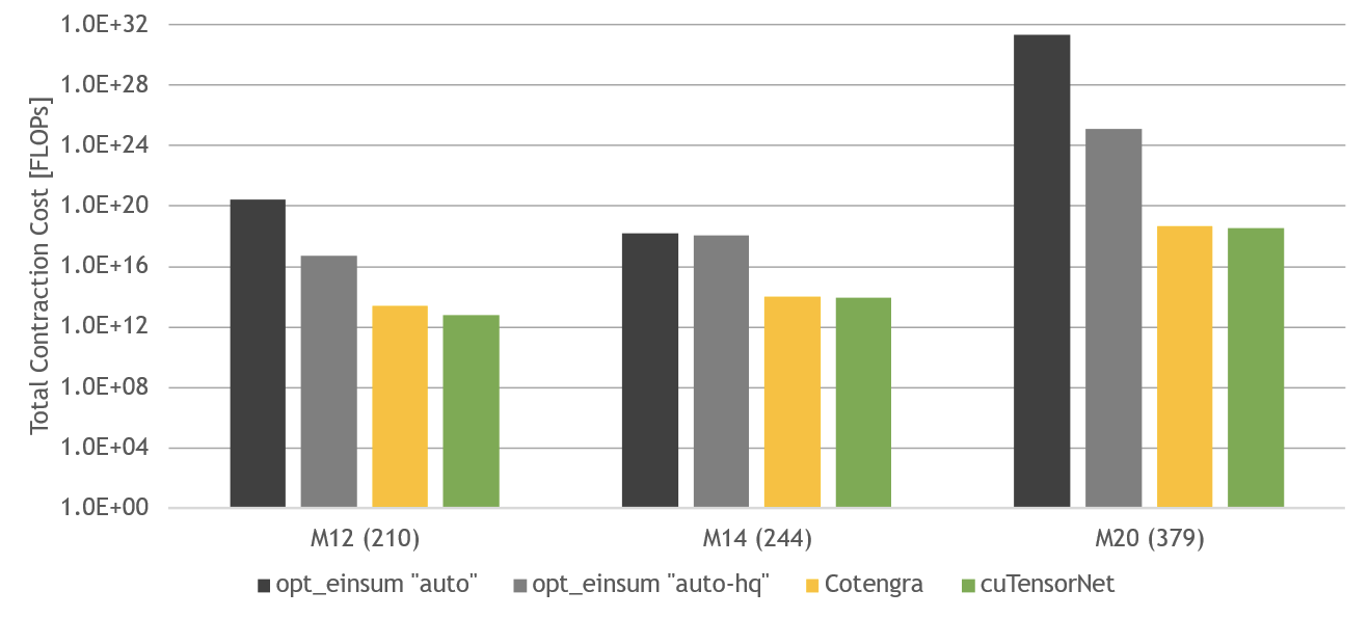
Bar chart shows that test circuits are random quantum circuits of depth 12, 14, and 20.
Figure 3. cuTensorNet pathfinding performance compared to similar packages, measured in FLOPs for the resulting contraction

cuTensorNet performs well compared to the opt_einsum library in finding an optimal path, and slightly better than Cotengra for these circuits.

cuTensorNet also finds a high-quality path quickly. The time taken to find a contraction for cuTensorNet compared to Cotengra is plotted in Figure 4, for the Sycamore quantum circuits problems with different depth. For the most complex problem with over 3,000 tensors in the network, cuTensorNet still finds its optimal path in just 40 seconds.
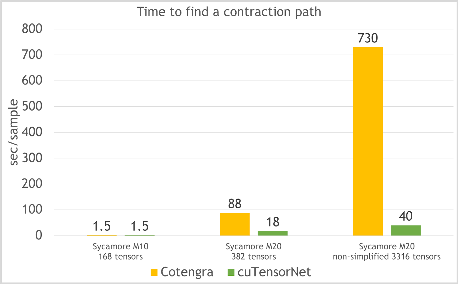
Bar chart shows that, for the largest instances of random quantum circuits, cuTensorNet finds an optimal path nearly 20x faster
Figure 4. Time to solution for cuTensorNet pathfinding, compared to Cotengra, for the Sycamore quantum circuits problems.

Execution

The execution component relies on the cuTENSOR library as the backend for efficient execution on the GPU. It consists of the following phases: 

  • Planning: The decision engine of the execution component. It analyzes the contraction path, deciding the best way to execute it on GPU using the minimal workspace. It also decides on the best kernels to be used for each of the pairwise contractions. 
  • Computation: This phase computes all the pairwise contractions using the cuTENSOR library.  
  • Autotuning: (Optional) Different kernels based on different heuristics are tried for pairwise contraction and the best is chosen. 

Execution performance

Figure 5 measures the speedup of the contraction execution for cuTensorNet compared to CuPy, for several different circuits. Depending on the circuit, cuTensorNet offers around an 8-20x speedup for the contraction execution.  
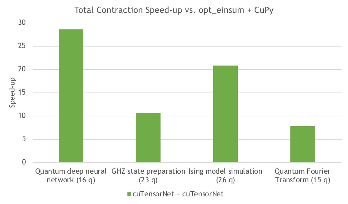
Bar chart shows that cuTensorNet offers roughly an 8–20x speedup in the contraction phase.
Figure 5. Contraction speedup of cuTensorNet vs. cuPy on a single A100 GPU, for several key quantum algorithms.

cuTensorNet example 

cuTensorNet provides both C and Python APIs that allow you to compute tensor network contractions efficiently without requiring any expertise on how to find the best contraction path or how to execute it on GPUs.  

High-level Python APIs 

cuTensorNet offers high-level Python APIs that are interoperable with NumPy and CuPy ndarrays and PyTorch tensors. For example, the einsum expression of a tensor network can be used in a single function call to contract. cuTensorNet performs all the required steps, returning the contracted network as a result. 

import cupy as cp
import cuquantum 
 
# Compute D_{m,x,n,y} = A_{m,h,k,n} B_{u,k,h} C_{x,u,y} 
# Create an array of extents (shapes) for each tensor 
extentA = (96, 64, 64, 96) 
extentB = (96, 64, 64) 
extentC = (64, 96, 64) 
extentD = (96, 64, 96, 64) 
 
# Generate input tensor data directly on GPU 
A_d = cp.random.random(extentA, dtype=cp.float32) 
B_d = cp.random.random(extentB, dtype=cp.float32) 
C_d = cp.random.random(extentC, dtype=cp.float32) 
 
# Set the pathfinder options 
options = cuquantum.OptimizerOptions() 
options.slicing.disable_slicing = 1  # disable slicing 
options.samples = 100                # number of hyper-optimizer samples 
 
# Run the contraction on a CUDA stream 
stream = cp.cuda.Stream() 
D_d, info = cuquantum.contract( 
    'mhkn,ukh,xuy->mxny', A_d, B_d, C_d, 
    optimize=options, stream=stream, return_info=True) 
stream.synchronize() 
 
# Check the optimizer info 
print(f"{info[1].opt_cost/1e9} GFLOPS") 

From this code example, you can see that all cuTensorNet operations are encapsulated in the single contract API. The output for this example is 14.495514624 GFLOPS: the number of floating-point operations estimated based on the contraction path found by the path finder. To perform the same steps manually, you can also use the cuQuantum.Network object.

Low-level APIs  

As previously discussed, the C and Python APIs are designed in a straightforward expressive fashion. You can call the pathfinder function to get an optimized path, followed by a call to perform the contraction on the GPU using that path.  

For advanced users, the cuTensorNet library API is designed to grant access to all algorithmic choices available to enable research in this field. For example, you can control how many hyper-optimizer samples the pathfinder can try to find the best contraction path.

There are dozens of parameters that you can modify or control. These are accessible through the helper functions and allow the simple functionalities API to remain unchanged. You are also allowed to provide your own path. For more information about the lower-level options and examples of how to use them, see cuquantum.Network.  

Summary

The cuTensorNet library of the NVIDIA cuQuantum SDK aims to accelerate tensor network computation on GPUs. In this post, we showed the speedup over state-of-the-art tensor network libraries on key quantum algorithms. 

There is extensive development to improve cuTensorNet and expand it with new algorithmic advancements as well as multi-node, multi-GPU execution.  

The cuTensorNet library goal is to provide a useful tool for groundbreaking developments in quantum computing. Have feedback and suggestions on how we can improve the cuQuantum libraries? Send email to cuquantum-feedback@nvidia.com

For more information, see the following resources: 

Categories
Misc

3 Methods for Speeding up AI Model Development with TAO Toolkit

How do you shorten your AI application’s TTM? Here are 3 methods to eliminate framework complexity and cut your training time in half using TAO Toolkit.
AI applications are powered by models. Deep learning models are built on mathematical algorithms and trained using data and human expertise. These models can accurately predict outcomes based on input data such as images, text, or speech.

Building, training, and optimizing these tasks are both critical and time-intensive. Domain expertise and countless hours of computation are needed to develop production-quality models. This is at odds with how quickly enterprises must operationalize their AI initiatives and reduce their time to market (TTM). 

Fine-tuning pretrained models without AI expertise

Fortunately, there is a solution: pretrained models. Using transfer learning, a pretrained model is one that has already been trained on representative datasets and fine-tuned with weights and biases. Unlike traditional AI algorithms that require significant time and resources to train, AI solutions built with pretrained models are delivered as fully operational, ready-to-use AI engines for a variety of use cases.

In most cases, an “out-of-box” pretrained model may not fit your use case or deliver the accuracy and performance you need. For these instances, you will have to modify or customize the pretrained model to fit your use-case needs.

Customizing pretrained models for different use cases

So how do you customize a pretrained model without spending too much time and effort? You can use NVIDIA TAO, an AI-model-adaptation framework, to simplify your development workflow. The TAO Toolkit is a CLI- and Jupyter notebook-based solution of NVIDIA TAO that makes it very easy to fine-tune pretrained models with your own data. No AI expertise is required. 

The TAO Toolkit is highly extensible and helps you adapt your model to new environments, augment your data, or add new classes.

Below are three examples highlighted in the NVIDIA whitepaper that explores proven methodologies for speeding up your AI workflow process.

  • Adapting to different camera types: Say you want to deploy a solution to infrared or thermal cameras. You can use the PeopleNet model that has already been trained on millions of images. Fine-tune it with only 2,500 images to achieve an mAP of almost 80%. 
  • Augmenting limited dataset: Data collection is time-consuming. With offline or online data augmentation, you can modify your dataset. Augmenting your dataset adds more variation and randomness that enables model generalization. This improves model accuracy on data the model has never seen before.
  • Adding new classes: Imagine that you have been asked to create an application that detects if people are wearing helmets while riding their bicycles. With the TAO Toolkit, you can use a model that detects people, and add a new “helmet class” to that model. Fine-tune it with the dataset that contains classes for both people and helmet. 

Put it into practice

When you eliminate AI framework complexity, you can focus on what matters: shortening your AI application’s TTM. The TAO Toolkit makes it incredibly easy for you to train, adapt and optimize pretrained models, without the need for large training datasets and AI expertise.

Visit the Github page to get started with the use cases described in the whitepaper. Learn more about the TAO Toolkit.

Categories
Misc

Validate Applications for Secure Edge Deployments with the Expanded NVIDIA Metropolis Partner Program

The Metropolis Partner Program expanded to include a certification that ensures partner applications can be securely deployed to any location with NVIDIA Fleet Command.

Building production-ready AI applications is hard, especially when starting from scratch. That’s why NVIDIA created Metropolis, a suite of tools to help developers build and bring to market vision AI applications. 

Deploying these applications in production, especially outside of the data center, can be just as difficult. For many organizations, determining the best way to deploy an application at customer sites is a task started after customer conversations are underway. The Metropolis Partner Program is addressing this with a certification that ensures partner applications can be securely deployed to any location with NVIDIA Fleet Command.

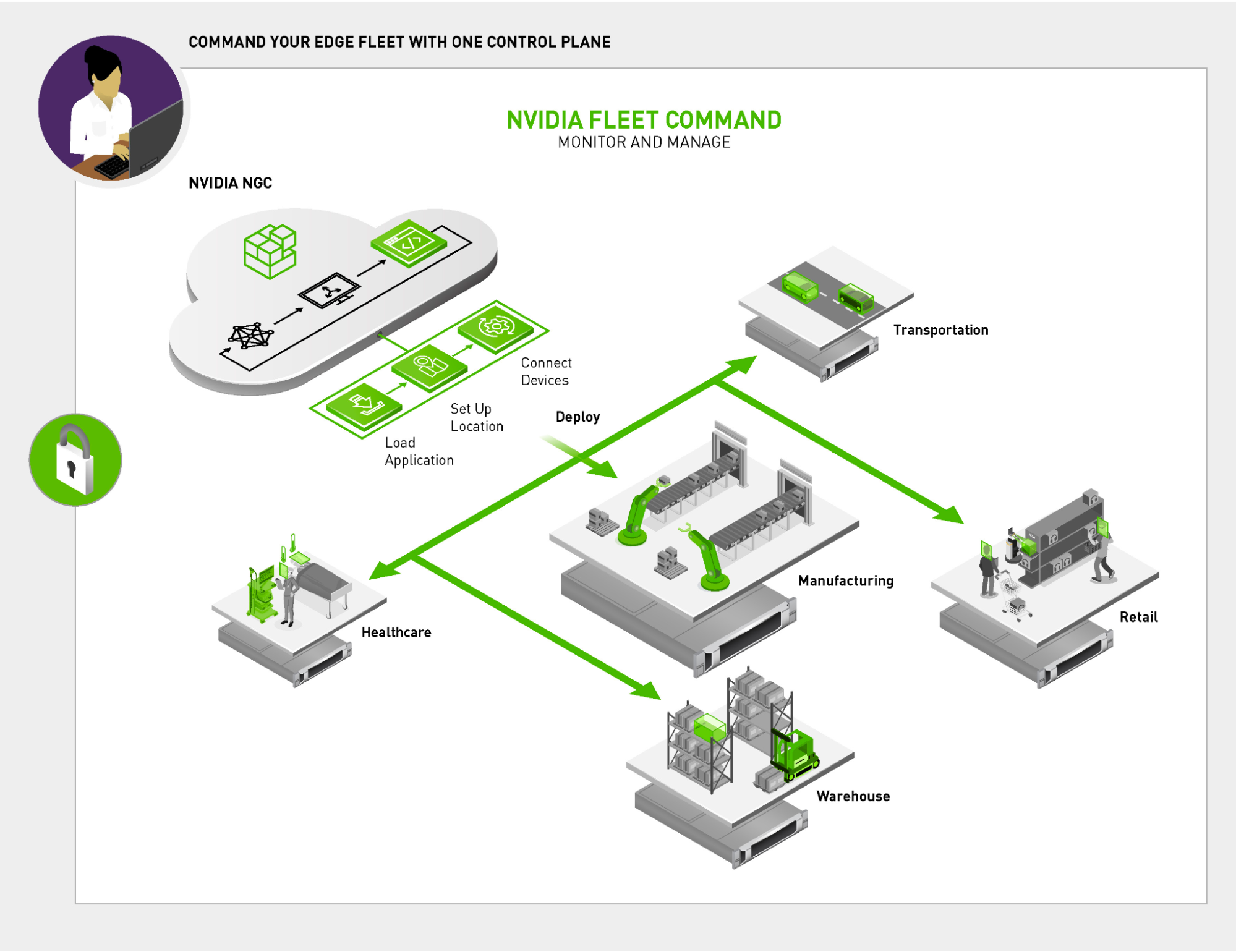
Fleet Command—a cloud service that centrally connects systems at edge locations—helps organizations securely deploy, manage, and scale AI applications from one dashboard. It’s the best way to orchestrate AI across hundreds or even thousands of devices covering vast physical distances. Now, Metropolis partners can use Fleet Command for free to deploy and scale their applications in production environments. 

A cloud representing Fleet Command is connected to several locations that represent various different types of locations across several industries including healthcare, retail, warehouse, manufacturing, and transportation.
Figure 1: Centrally manage AI application deployments across all of your edge locations with Fleet Command.

Deploying an application using Fleet Command gives partners a platform to easily conduct POCs at customer sites. This can be done without building custom tools to get applications operational in unique customer environments. Additionally, after the evaluation is complete, the partner has all of the necessary infrastructure to easily scale an application from an evaluation environment to the entire production environment. Saving time gives partners the freedom to focus all their resources on building valuable AI applications.

Once an application is ready for deployment on Fleet Command, partners have free access to the platform for a year. The platform includes cloud access to servers with the latest NVIDIA GPUs, and NVIDIA experts on AI and optimizations, amounting to over a $100,000 value. 

Partners looking to demonstrate the value of their application to customers have access to NVIDIA LaunchPad. LaunchPad provides enterprises immediate, short-term access to all of the features and functionality of Fleet Command including provisioning edge infrastructure, deploying and managing applications, and monitoring their edge fleet. Partners can use Fleet Command on LaunchPad for customers to experience the application in an isolated environment before moving to a full evaluation in a production setting. 

Over 50 Metropolis Partner Program members are integrating their applications to be deployed and managed on Fleet Command. Partners include Milestone for AI-enabled video management software, OSARO for efficient pick and place robotics solutions, and IronYun for intelligent video analytics in smart buildings.

“With NVIDIA Fleet Command, we can easily deploy and manage our vision AI apps across the edge infrastructure in minutes rather than days,” said Paul Sun, CEO of IronYun.  “Our sales and testing cycles are drastically reduced.”

The Metropolis Partner Program enables AI developers with tools to streamline every stage of the process to acquire and keep new customers. This ranges from application development on Metropolis to demos and evaluations on LaunchPad, to POCs and deployments on Fleet Command.

Get access to Fleet Command and LaunchPad today by applying to join the Metropolis Partner Program. If you’re already a member, reach out to your representative to learn how to get started.

Categories
Misc

Podsplainer: What’s a Recommender System? NVIDIA’s Even Oldridge Breaks It Down

The very thing that makes the internet so useful to so many people — the vast quantity of information that’s out there — can also make going online frustrating. There’s so much available that the sheer volume of choices can be overwhelming. That’s where recommender systems come in, explains NVIDIA AI Podcast host Noah Kravitz. Read article >

The post Podsplainer: What’s a Recommender System? NVIDIA’s Even Oldridge Breaks It Down appeared first on NVIDIA Blog.

Categories
Misc

Conversion of SVC with RBF Kernel to Tensorflow model?

Is there a way to convert support vector classifier with rbf kernel to tf model?

I am aware of converting support vector classifier with linear kernel because there exists coef_ where we can find parameters and assign to tf model. Got this idea from how to convert saved model from sklearn into tensorflow/lite.

However _coef wont be there for rbf , so i am not sure on how to convert this model to an tf model.

Any suggestions are highly helpful. Thanks

submitted by /u/Mother-Beyond9493
[visit reddit] [comments]

Categories
Misc

[TFLite] Mozilla + Coqui Speech Technology Hackathon

[TFLite] Mozilla + Coqui Speech Technology Hackathon submitted by /u/josh-r-meyer
[visit reddit] [comments]
Categories
Misc

Tensorflow-GPU=2.6.0 and cudatoolkit >=11 with conda

I have a problem, which I could not solve yet.

I need to create a conda environment with tensorflow=2.6.0, python=3.8 and cudatoolkit>=11 (using ampere GPU)

I cannot use conda default channel. Until now I tried using conda-forge and nvidia channel.

I have not succeeded in creating a conda environment with the above requirements. Anyone got a hint?

The machine got centos with Nvidia driver 495 and cuda 11.5

submitted by /u/alex_bababu
[visit reddit] [comments]

Categories
Misc

classify known images and reject unknown images; Resnet50?

I am trying to build a sorting system to sort parts by taking a picture of the part, identifying the part, and then telling a robot to move the part into the appropriate bucket. 99% of the parts are known and can be trained for. 1% of the parts are not known. I would like the known parts to be put in their buckets, and all of the unknown parts to be rejected into a single bucket called unknown.

I naively thought I would be able to do this with Resnet50 by looking at the weights returned in the prediction array. I thought the predictor would have uncertainty when presented with an unknown part. However, I have discovered that Resnet50 (and perhaps all image classifiers) will force any image to be in one of it’s trained for buckets with a high level of confidence.

Because only 1% of the parts are unknown, I can’t realistically gather enough of them to train for. Furthermore, I don’t know when and where they will show up.

Does anyone know of a technique I could use to sort images of known parts into their buckets, and reject unknown parts?

submitted by /u/marlon1492
[visit reddit] [comments]

Categories
Misc

(beginner) am I doing something wrong is it supposed to take this long to import TensorFlow into ide

I am using Dataspell and have a jupyter notebook set up inside dataspell, I’ve done simple imports such as

import TensorFlow as tf
import tensorflow_hub as hub
import tensorflow_text as text

but its has been like 2 hours and it still hasn’t finished loading, I’ve made sure that i already installed the packages using terminal pip install TensorFlow etc

submitted by /u/ratmanreturns265
[visit reddit] [comments]

Categories
Misc

Saving Time and Money in the Cloud with the Latest NVIDIA-Powered Instances

The greater performance delivered by current-generation NVIDIA GPU-accelerated instances more than outweighs the per-hour pricing differences of prior-generation GPUs.
AI is transforming every industry, enabling powerful new applications and use cases that simply weren’t possible with traditional software. As AI continues to proliferate, and with the size and complexity of AI models on the rise, significant advances in AI compute performance are required to keep up.

That’s where the NVIDIA platform comes in.

With a full-stack approach spanning chips, systems, software, and even the entire data center, NVIDIA delivers both the highest performance and the greatest versatility for all AI workloads, including AI training. NVIDIA demonstrated this in the MLPerf Training v1.1, the latest edition of an industry-standard, peer-reviewed benchmark suite that measures ML training performance across a wide range of networks. Systems powered by the NVIDIA A100 Tensor Core GPU, including the Azure NDm A100 v4 cloud instance, delivered chart-topping results, set new records, and were the only ones to complete all eight MLPerf Training tests.

All major cloud service providers offer NVIDIA GPU-accelerated instances powered by the A100, making the public cloud a great place to tap into the performance and capabilities of the NVIDIA platform.  In this post, I show how a strategy of selecting current-generation instances based on the A100 not only delivers the fastest time to train AI models in the cloud but is also the most cost-effective.

NVIDIA A100 turbocharges AI training

The NVIDIA A100 is based on the Ampere architecture, which incorporates a host of innovations that speed up AI training compared to the prior-generation NVIDIA V100, such as third-generation Tensor Cores, a new generation of NVLink, and much greater memory bandwidth. These enhancements deliver a giant performance leap, enabling the reduction in the time to train a wide range of AI networks.

In this post, I use ResNet-50 to represent image classification, BERT Large for natural language processing, and DLRM for recommender systems.

Chart shows the performance speed-ups of the NVIDIA A100 40GB vs the NVIDIA V100 32GB in DLRM, BERT Large fine tuning, and ResNet-50. They are 2X, 2.6X, and 1.5X, respectively.
Figure 1. The NVIDIA A100 dramatically reduces the time to train AI models compared to the NVIDIA V100

GPU Server: Dual socket AMD EPYC 7742 @ 2.25GHz w/ 8x NVIDIA A100 SXM4-40GB and Dual socket Intel Xeon E5-2698 v4 @ 2.2GHz w/ 8x NVIDIA V100 SXM2-32GB.  Frameworks: TensorFlow for ResNet-50 v1.5, PyTorch for BERT-Large and DLRM; Precision: Mixed+XLA for ResNet-50 v1.5, Mixed for BERT-Large and DLRM.  NVIDIA Driver: 465.19.01; Dataset: ImageNet2012 for ResNet-50 v1.5, SQuaD v1.1 for BERT Large Fine Tuning, Criteo Terabyte Dataset for DLRM, Batch sizes for ResNet-50: A100, V100 = 256; Batch sizes for BERT Large: A100 = 32, V100 = 10; Batch sizes for DLRM: A100, V100 = 65536.

Faster training times speed time to insight, maximizing the productivity of an organization’s data science teams and getting the trained network deployed sooner. There’s also another important benefit: lower costs!

Cloud instances are commonly priced per unit of time, with hourly pricing typical for on-demand usage. The cost to train a model is the product of both hourly instance pricing and the time required to train a model.

Although it can be tempting to select the instances with the lowest hourly price, this might not lead to the lowest cost to train. An instance might be slightly cheaper on a per-hour basis but take significantly longer to train a model. The total cost to train is higher than it would be with the higher-priced instance that gets the job done more quickly. In addition, there’s the time lost waiting for the slower instance to complete the training run.

In the performance numbers shown earlier, the NVIDIA A100 can train models much more quickly than NVIDIA V100. That’s almost 3x as fast in the case of BERT Large Fine Tuning. At the same time, A100-based instances from major cloud providers are often only priced at modest premiums to their prior-generation, V100-based counterparts.

In this post, I discuss how using A100-based cloud instances enables you to save time and money while training AI models, compared to V100-based cloud instances.

Translating performance into savings

Given the immense computational demands of AI training, it is common to train models using multiple GPUs working in concert to reduce training times significantly.

The NVIDIA platform has been designed to deliver industry-leading per-accelerator performance and achieve the best performance and highest ROI at scale, thanks to technologies like NVLink and NVSwitch. That’s why, in this post, I estimate the cost savings that instances with eight NVIDIA A100 GPUs can deliver compared to instances with eight NVIDIA V100 GPUs.

For this analysis, I estimate the relative costs to train ResNet-50, fine tune BERT Large, and train DLRM on V100- and A100-based instances from three major cloud service providers: Amazon Web Services, Google Cloud Platform, and Microsoft Azure.

CSP Instance GPU Configuration
Amazon Web Services p4d.24xlarge 8x NVIDIA A100 40GB
p3dn.24xlarge 8x NVIDIA V100 32GB
p3.16xlarge 8x NVIDIA V100 16GB
Google Cloud Platform a2-highgpu-8g 8x NVIDIA A100 40GB
n1-highmem-96 8x NVIDIA V100 16GB
Microsoft Azure Standard_ND96asr_v4 8x NVIDIA A100 40GB
ND40rs v2 8x NVIDIA V100 32GB
Table 1. NVIDIA GPU-accelerated instances from AWS, GCP, and Microsoft Azure.

Estimate methodology

To estimate the training performance of the cloud instances, I used measured time to train data on NVIDIA DGX systems with GPU configurations that correspond to those in the instances. As a result of the deep engineering collaboration with these cloud partners, the performance of NVIDIA-powered cloud instances should be similar to the performance achievable on the DGX systems.

Then, with the measured time-to-train data, I used on-demand, per-hour instance pricing to estimate the cost to train ResNet-50, fine tune BERT Large, and train DLRM. 

Estimated cost savings

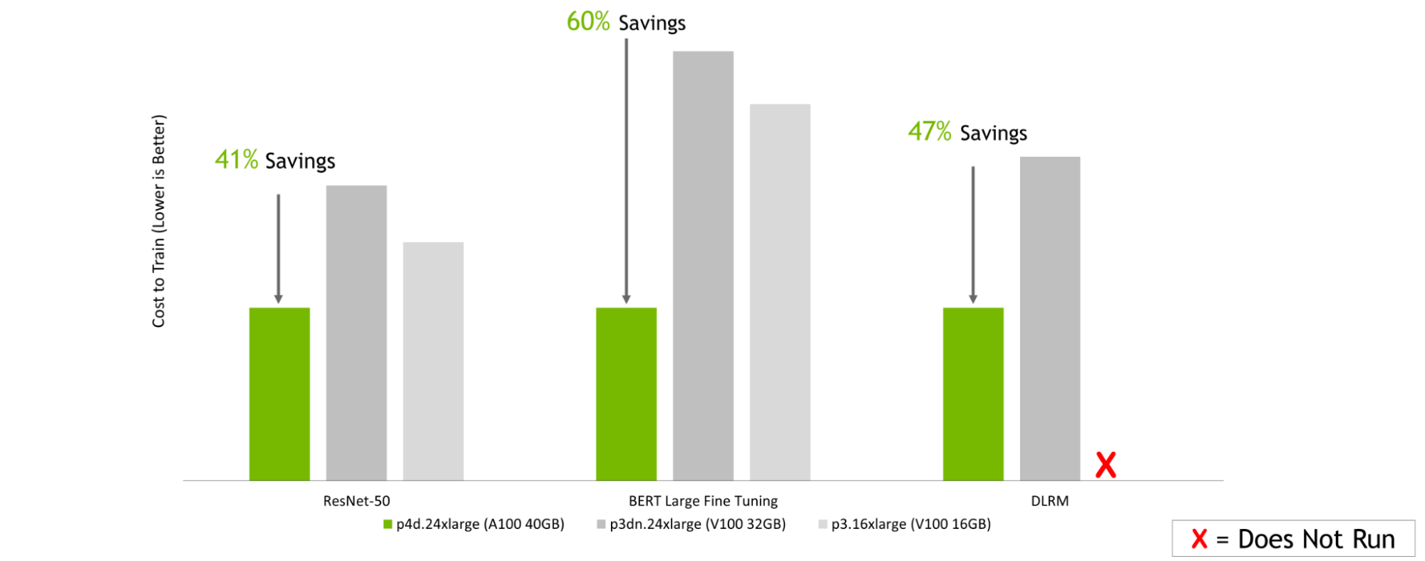
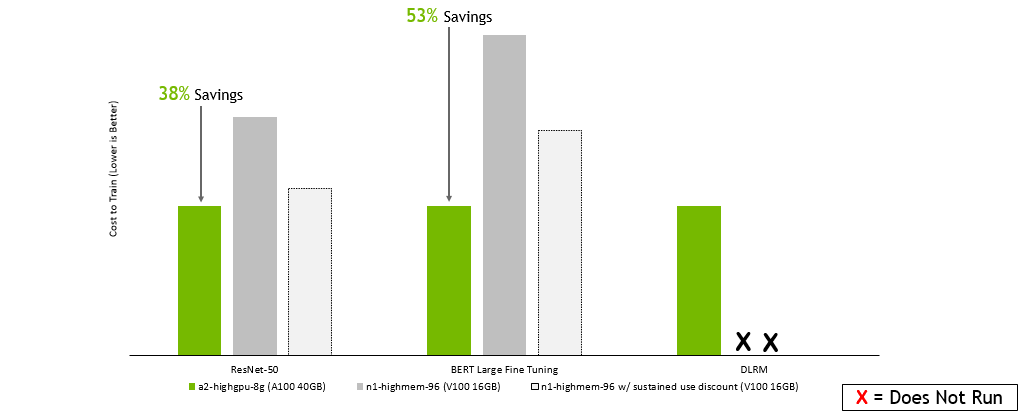
The following charts all tell a similar story: no matter which cloud service provider you choose, selecting instances based on the latest NVIDIA A100 GPUs can translate into significant cost savings when training a range of AI models. This is even though, on a per-hour basis, instances based on the NVIDIA A100 are more expensive than instances using prior-generation V100 GPUs.

Amazon Web Services:

Chart shows the relative estimated cost to train ResNet-50, BERT Large Fine Tuning, and DLRM on AWS instances based on NVIDIA GPUs: p3.16xlarge (V100 16GB), p3dn.24xlarge (V100 32GB), and p4d.24xlarge (A100 40GB). Estimated savings with A100 = 41% for ResNet-50, 60% for BERT Large Fine Tuning, and 47% for DLRM.
Figure 2. Estimated cost savings for training models using A100 instances on AWS compared to V100 (16GB and 32GB) instances

GPU Server: Dual socket AMD EPYC 7742 @ 2.25GHz w/ 8x NVIDIA A100 SXM4-40GB, Dual socket Intel Xeon E5-2698 v4 @ 2.2GHz w/ 8x NVIDIA V100 SXM2-32GB, and Dual socket Intel Xeon E5-2698 v4 @ 2.2GHz w/ 8x NVIDIA V100 SXM2-16GB.  Frameworks: TensorFlow for ResNet-50 v1.5, PyTorch for BERT-Large and DLRM; Precision: Mixed+XLA for ResNet-50 v1.5, Mixed for BERT-Large and DLRM.  NVIDIA Driver: 465.19.01; Dataset: Imagenet2012 for ResNet-50 v1.5, SQuaD v1.1 for BERT Large Fine Tuning, Criteo Terabyte Dataset for DLRM, Batch sizes for ResNet-50: A100, V100 = 256; Batch sizes for BERT Large: A100 = 32, V100 = 10; Batch sizes for DLRM: A100, V100 = 65536; Cost estimated using performance data run on the earlier configurations as well as on-demand instance pricing as of 2/8/2022.

Google Cloud Platform:

Chart shows the relative estimated cost to train ResNet-50, BERT Large Fine Tuning, and DLRM on GCP instances based on NVIDIA GPUs: a2-highgpu-8g (A100 40GB), n1-highmem-96 (V100 16GB), and n1-highmem-96 with a sustained use discount applied. Estimated savings with A100 = 38% for ResNet-50 and 53% for BERT Large Fine Tuning.
Figure 3. Estimated cost savings for training models using A100 instances on GCP compared to V100 (16GB) instances

GPU Server: Dual socket AMD EPYC 7742 @ 2.25GHz w/ 8x NVIDIA A100 SXM4-40GB, Dual socket Intel Xeon E5-2698 v4 @ 2.2GHz w/ 8x NVIDIA V100 SXM2-32GB, and Dual socket Intel Xeon E5-2698 v4 @ 2.2GHz w/ 8x NVIDIA V100 SXM2-16GB.  Frameworks: TensorFlow for ResNet-50 v1.5, PyTorch for BERT-Large and DLRM; Precision: Mixed+XLA for ResNet-50 v1.5, Mixed for BERT-Large and DLRM.  NVIDIA Driver: 465.19.01; Dataset: ImageNet2012 for ResNet-50 v1.5, SQuaD v1.1 for BERT Large Fine Tuning, Criteo Terabyte Dataset for DLRM, Batch sizes for ResNet-50: A100, V100 = 256; Batch sizes for BERT Large: A100 = 32, V100 = 10; Batch sizes for DLRM: A100, V100 = 65536; Cost estimated using performance data run on the earlier configurations as well as on-demand instance pricing as of 2/8/2022.

Microsoft Azure:

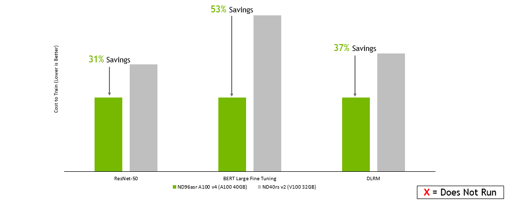
Chart shows the relative estimated cost to train ResNet-50, BERT Large Fine Tuning, and DLRM on Azure instances based on NVIDIA GPUs: ND96asr A100 v4 (A100 40GB) and ND40rs v2 (V100 16GB). Estimated savings with A100 = 31% for ResNet-50, 53% for BERT Large Fine Tuning, and 37% for DLRM.
Figure 4. Estimated cost savings for training models using A100 instances on GCP compared to V100 (32-GB) instances

GPU Server: Dual socket AMD EPYC 7742 @ 2.25GHz w/ 8x NVIDIA A100 SXM4-40GB, Dual socket Intel Xeon E5-2698 v4 @ 2.2GHz w/ 8x NVIDIA V100 SXM2-32GB, and Dual socket Intel Xeon E5-2698 v4 @ 2.2GHz w/ 8x NVIDIA V100 SXM2-16GB.  Frameworks: TensorFlow for ResNet-50 v1.5, PyTorch for BERT-Large and DLRM; Precision: Mixed+XLA for ResNet-50 v1.5, Mixed for BERT-Large and DLRM.  NVIDIA Driver: 465.19.01; Dataset: ImageNet2012 for ResNet-50 v1.5, SQuaD v1.1 for BERT Large Fine Tuning, Criteo Terabyte Dataset for DLRM, Batch sizes for ResNet-50: A100, V100 = 256; Batch sizes for BERT Large: A100 = 32, V100 = 10; Batch sizes for DLRM: A100, V100 = 65536; Costs estimated using performance data run on the earlier configurations as well as on-demand instance pricing as of 2/8/2022.

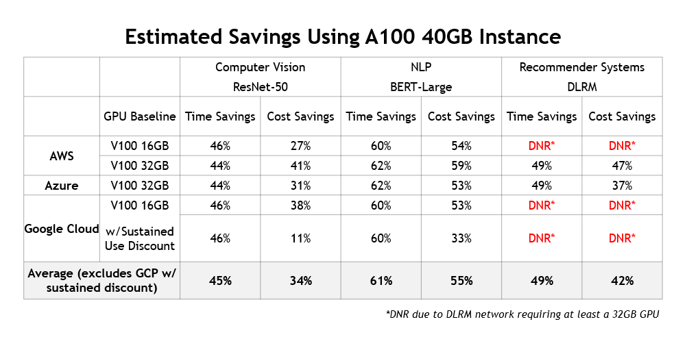
In addition to delivering lower training costs and saving users a significant amount of time, there’s another benefit to using current-generation instances:  they enable fundamentally new AI use cases. For example, AI-based recommendation engines are becoming increasingly popular and NVIDIA GPUs are commonly used to train them. Figure 5 summarizes the cost and time savings that A100-instances deliver across different cloud providers:

Table summarizes the estimated time and cost benefits of using cloud instances with the NVIDIA A100 40GB GPU compared to instances with NVIDIA V100 16GB and V100 32GB GPUs.
Figure 5. Time and cost savings of A100-based instances compared to V100 counterparts. Based on on-demand instance pricing as of 2/8/2022.

Higher performance also means higher savings

These results presented here show that the much greater performance delivered by current-generation NVIDIA GPU-accelerated instances more than outweighs the per-hour pricing differences compared to older instances that use prior-generation GPUs.

Instances based on the latest NVIDIA A100 GPUs not only maximize the productivity of your data science teams by minimizing training time, but they’re also the most cost-effective way to train your models in the cloud.

To learn more about the many options for using NVIDIA acceleration in the cloud, see Cloud Computing.