Lets say for object detection of a video feed, would there be any value in using Google Coral Edge USB TPUs or processing Tensorflow on a Jetson device if the alterantive is something like an Intel NUC 10 i7 ( Core i7-10710U Passmark score: 10.1k) with NVME storage?
SIGGRAPH 2021 is the premier conference and exhibition in computer graphics and interactive techniques. This year, participants can join a series of exciting pre-conference webinars called SIGGRAPH Frontiers Interactions.
Add SIGGRAPH Frontiers to Your Calendar – Courses Begin May 24th
SIGGRAPH 2021 is the premier conference and exhibition in computer graphics and interactive techniques. This year, participants can join a series of exciting pre-conference webinars called SIGGRAPH Frontiers Interactions. Starting on May 24, you can take part in industry-leading discussions around ray tracing, machine learning and neural networks.
These pre-conference webinars are ongoing educational events that will take place through June 18, and feature several NVIDIA guest speakers. Both courses are free. Simply add the events to your calendar of choice here and show up to experience the research deep dive and industry-leading discourse.
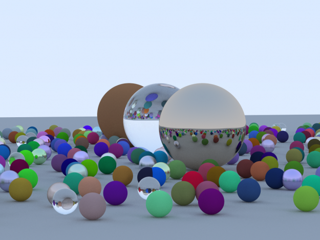
Introduction to Ray Tracing Course
The first of seven ray tracing webinars starts on May 25, and features Peter Shirley, author of the popular book, Ray Tracing in One Weekend. This is a great introductory level course to gain a strong understanding of the basic principles of ray tracing. Other interactive lectures feature experts from Disney Animation and NVIDIA.
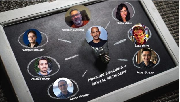
Machine Learning and Neural Networks Course
The first of seven machine learning and neural network webinars starts on May 24. Several ML and NN experts from Google, Disney, Apple and NVIDIA will be featured. These are intermediate level courses intended to gain a strong understanding of the basic principles of ML and NN, and how it can be applied to your engineering solutions.
Make sure to stay up-to-date with all things SIGGRAPH and register for the virtual event, taking place August 9-13.
Researchers from the Netherlands’ University of Groningen have used AI to reveal that the Great Isaiah Scroll — the only entirely preserved volume from the original Dead Sea Scrolls — was likely copied by two scribes who wrote in a similar style.
Researchers from the Netherlands’ University of Groningen have used AI to reveal that the Great Isaiah Scroll — the only entirely preserved volume from the original Dead Sea Scrolls — was likely copied by two scribes who wrote in a similar style.
While most scholars long believed the Isaiah Scroll’s 17 sheets of parchment were copied by a single scribe around the second century BCE, others suggested that it was the work of two scribes who each wrote half the text.
These theorists “would try to find a ‘smoking gun’ in the handwriting, for example, a very specific trait in a letter that would identify a scribe,” said Mladen Popović, director of the University of Groningen’s Qumran Institute, which is dedicated to the study of the Dead Sea Scrolls.
But even a single scribe’s writing could have some natural variation across the text, caused by fatigue, injury, or even a change in writing implements. And analyzing these variations by traditional paleographic methods is impractical for a text as lengthy as the Isaiah Scroll, which contains more than 5,000 occurrences of just the letter aleph, or “a.”
Popović and his collaborators thought AI could help process the rich data from a digital copy of the text. In a recent PLOS One article, the team details how they used pattern recognition and AI techniques to pinpoint an area halfway through the scroll where there is an apparent transition from one scribe’s handwriting to another’s.
The analysis identified subtle differences in the positioning, thickness, and length of certain strokes in the first and second halves of the scroll.
After using an artificial neural network to separate the inked letters from the parchment on images of the Isaiah Scroll, the team used a Kohonen network, a type of unsupervised learning model, to collect multiple examples of the same characters in the text.
Precisely capturing the original writing “is important because the ancient ink traces relate directly to a person’s muscle movement and are person-specific,” said Lambert Schomaker, paper co-author and professor at the University of Groningen.
The group ran the neural networks using CUDA and NVIDIA GPUs in the university’s Peregrine HPC cluster, which includes over 200,000 CUDA cores.
To help check their results, the researchers added extra noise to the data, and found the AI analysis still came to the same conclusion. They also created heat maps that averaged how individual characters appeared in the first and second halves of the scroll, helping scholars visualize the difference between the sections.
The researchers plan to apply this methodology to additional parchments that make up the Dead Sea Scrolls.
“We are now able to identify different scribes,” said Popović.”We will never know their names. But after seventy years of study, this feels as if we can finally shake hands with them through their handwriting.”
For a particle physicist, the world’s biggest questions — how did the universe originate and what’s beyond it — can only be answered with help from the world’s smallest building blocks. James Kahn, a consultant with German research platform Helmholtz AI and a collaborator on the global Belle II particle physics experiment, uses AI and Read article >
Legendary car manufacturer Aston Martin is using the latest virtual and mixed reality technologies to drive new experiences for customers and designers. The company has worked with Lenovo to use VR and AR to deliver a unique experience that allowed customers to explore its first luxury SUV, the Aston Martin DBX, without physically being in Read article >
NVIDIA will deliver a double-barrelled keynote packed with innovations in AI, the cloud, data centers and gaming at Computex 2021 in Taiwan, on June 1. NVIDIA’s Jeff Fisher, senior vice president of GeForce gaming products, will discuss how NVIDIA is addressing the explosive growth in worldwide gaming. And Manuvir Das, head of enterprise computing at Read article >
Wondering if anyone has insight into how to run both TF 1.x and TF 2.x in the same python program. I understand that its possible to use
import tensorflow.compat.v1 as tf
tf.disable_v2_behavior()
but my use case might be a bit different. Basically I’m using a forked gpt-2-simple github repo which is fully written in tf 1.x and within the same program i need to utilize tf hub which is obviously only in tf 2.x.
If anyone know if/how these two versions can run in unison I think that would be very helpful and insightful to the community as well.
*Insert snide comment about how many issues tf 2.x has caused me*
Game developers around the world attended GTC to experience how the latest NVIDIA technologies are creating realistic graphics and interactive experiences in gaming. Catch up on the top sessions available on NVIDIA On-Demand now.
Game developers around the world attended GTC to experience how the latest NVIDIA technologies are creating realistic graphics and interactive experiences in gaming.
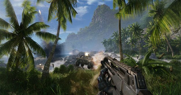
We showcased the NVIDIA-powered tools that deliver stunning graphics and improved game performance, and how developers are integrating that technology into popular game titles such as Minecraft, Cyberpunk 2077, LEGO Builder’s Journey, and more. All of these GTC sessions are now available through NVIDIA On-Demand, so you can catch up on the latest tools and techniques in game development, from real-time ray tracing to low-latency software development kits.
Ray Tracing in One Weekend
Watch this session to get a beginners introduction to ray tracing. Peter Shirley, author of the popular book, Ray Tracing in One Weekend, showed audiences how to use ray tracing to create amazing images.
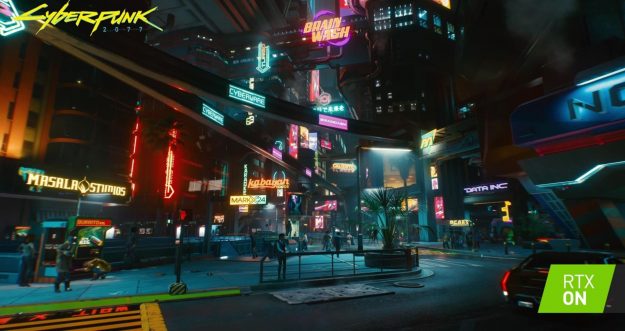
Cyberpunk 2077 is a role-playing game set in Night City, a futuristic megalopolis full of contrasts, shadows, reflections, and radiant neons. Learn about the challenges of creating the graphics for Night City, and how the team approached the game lighting for Cyberpunk 2077.
Get insights into the work that went into delivering RTX features in one of the greatest games of all time, from adding support for ray tracing without having to port the entire DX11 engine, to the ins-and-outs of how the team got NVIDIA DLSS to work.
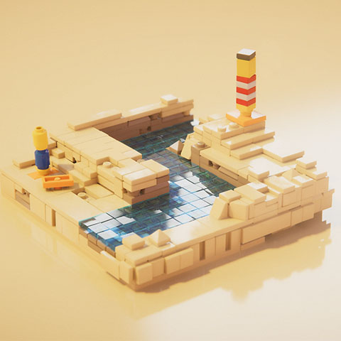
LEGO Builder’s Journey: Rendering Realistic LEGO Bricks using Ray Tracing in Unity
Learn how LEGO dioramas were rendered in real time using Unity high-definition render pipeline and ray tracing. From lighting and materials to geometry processing and post effects, get an inside look into how the team got as close to realism as possible in a limited time. During this talk, we announced that NVIDIA DLSS will be natively integrated into Unity by the end of the year.
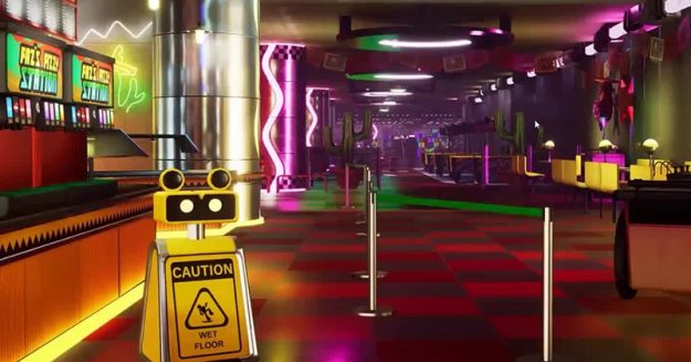
Learn how Steelwool Game and NVIDIA worked closely to develop and implement RTXGI for Five Nights at Freddy’s: Security Breach. This session dives into the use of RTXGI, and using ray tracing on modern hardware.

 SIGGRAPH 2021 is the premier conference and exhibition in computer graphics and interactive techniques. This year, participants can join a series of exciting pre-conference webinars called SIGGRAPH Frontiers Interactions.
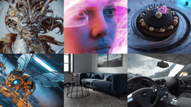
 Researchers from the Netherlands’ University of Groningen have used AI to reveal that the Great Isaiah Scroll — the only entirely preserved volume from the original Dead Sea Scrolls — was likely copied by two scribes who wrote in a similar style.
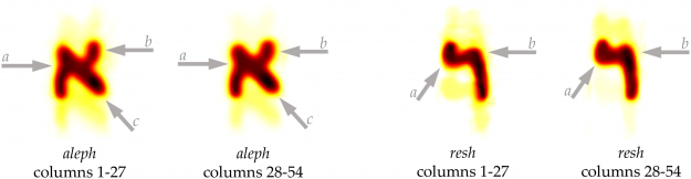


 Game developers around the world attended GTC to experience how the latest NVIDIA technologies are creating realistic graphics and interactive experiences in gaming. Catch up on the top sessions available on NVIDIA On-Demand now.