Meet Paige Frank: Avid hoopster, Python coder and robotics enthusiast. Still in high school, the Pittsburgh sophomore is so hooked on AI and robotics, she’s already a mentor to other curious teens. “Honestly, I never was that interested in STEM. I wanted to be a hair stylist as a kid, which is also cool, but Read article >
A rising technology star in Southeast Asia just put a sparkle in its AI. Vingroup, Vietnam’s largest conglomerate, is installing the most powerful AI supercomputer in the region. The NVIDIA DGX SuperPOD will power VinAI Research, Vingroup’s machine-learning lab, in global initiatives that span autonomous vehicles, healthcare and consumer services. One of the lab’s most Read article >
Artists and engineers, architects, and automakers are coming together around a new standard — born in the digital animation industry — that promises to weave all our virtual worlds together. That’s the conclusion of a group of panelists from a wide range of industries who gathered at NVIDIA GTC21 this week to talk about Pixar’s Read article >
To help developers hone their craft, NVIDIA this week introduced more than 50 new and updated tools and training materials for data scientists, researchers, students and developers of all kinds. The offerings range from software development kits for conversational AI and ray tracing, to hands-on courses from the NVIDIA Deep Learning Institute. They’re available to Read article >
This year, everyone can learn how to develop safe, robust autonomous vehicles on NVIDIA DRIVE. The annual DRIVE Developer Days is taking place April 20-22 during GTC 2021, featuring a series of specialized sessions on autonomous vehicle hardware and software, including perception, mapping, simulation and more, all led by NVIDIA experts. And now, registration is … Continued
This year, everyone can learn how to develop safe, robust autonomous vehicles on NVIDIA DRIVE.
The annual DRIVE Developer Days is taking place April 20-22 during GTC 2021, featuring a series of specialized sessions on autonomous vehicle hardware and software, including perception, mapping, simulation and more, all led by NVIDIA experts. And now, registration is free and open to all.
In the past, these AV developer sessions have been limited to NVIDIA customers. However, this year we are making these deep dive sessions available to all developers, with lessons learned by the NVIDIA team, as the need for AV systems is more apparent than ever before.
You can view the entire DRIVE Developer Day playlist by clicking here. Make sure youregister now to access these and 150+ autonomous vehicle sessions at GTC 2021.
Over the past couple of years, NVIDIA and NASA have been working closely on accelerating data science workflows using RAPIDS, and integrating these GPU-accelerated libraries with scientific use cases. This is the second post in a series that will discuss the results from an air pollution monitoring use case conducted during the COVID-19 pandemic, and … Continued
Over the past couple of years, NVIDIA and NASA have been working closely on accelerating data science workflows using RAPIDS, and integrating these GPU-accelerated libraries with scientific use cases. This is the second post in a series that will discuss the results from an air pollution monitoring use case conducted during the COVID-19 pandemic, and share code snippets to port existing CPU workflows to RAPIDS on NVIDIA GPUs. This first post of this series, we covered Accelerated Simulation of Air Pollution.
Monitoring the Decline of Air Pollution Across the Globe During the COVID-19 Pandemic
Another air quality application leveraging XGBoost and RAPIDS is the live monitoring of air quality through the combination of surface monitoring data and near real-time model data produced by the NASA GEOS-CF model. This approach is particularly useful to detect and quantify air pollution anomalies, i.e., patterns in air quality observations that cannot be explained by the model. The most prominent (and extreme) example of this is the decline of air pollution in the wake of the COVID-19 pandemic. As a result of the stay-at-home orders, traffic emissions of air pollutants such as nitrogen dioxide (NO2) decreased significantly, as apparent from both satellite observations and surface monitoring data. However, exactly quantifying the impact of COVID-19 restrictions on surface air quality solely based on these atmospheric observations is very difficult given that many other factors impact surface air pollution, including weather, chemistry, or wildfires.
Video 1. Daily nitrogen dioxide (NO2) measurements and percentage difference from a baseline model. Credits: Christoph Keller and NASA’s Scientific Visualization Studio.
The study conducted by Christoph and his colleagues fuses millions of observations – taken at 4,778 monitoring sites in 47 countries – with co-located model output produced by GEOS-CF. The sample code found at the covid_no2 repo, demonstrates the application for 10 selected cities (New York, Washington DC, San Francisco, Los Angeles, Beijing, Wuhan, London, Paris, Madrid, and Milan). The air quality observations for years 2018 through 2020 at these cities were obtained from the OpenAQ database (https://openaq.org/#/) and the European Environment Agency EEA (https://discomap.eea.europa.eu/map/fme/AirQualityExport.htm) and pre-processed into a single file for convenience:
Similarly, we preprocessed the GEOS-CF model output by subsampling the gridded native output (available in netCDF format at https://portal.nccs.nasa.gov/datashare/gmao/geos-cf/v1/das/) to the observation locations and saved the corresponding data as a table in text format that can be read similarly to the observation data:
The model data contains not only model predicted NO2 concentrations but also a number of ancillary model variables, such as information about the local weather and atmospheric composition (as taken from GEOS-CF) or calendar information.
The model data is then combined with the surface observation data to build an XGBoost bias-correction model that relates the model NO2 prediction to the observations. This is to account for the fact that the model prediction can be systematically different from the observations, e.g., because the model output represents the average over a 25×25 km2 domain while the surface observation is typically much more local in nature.
To train the XGBoost model, the model data is merged with the observations and the model bias is calculated from the merged data set to provide the label for the training (see sample code in repository mentioned above for full example):
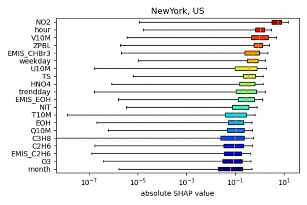
As shown in the figure below, the SHAP values for New York indicate that the most important predictors for the NO2 model bias (relative to the actual observation) is NO2 itself, followed by the hour of the day, wind speed (V10M) and the height of the planetary boundary layer (ZPBL). (note: to output the SHAP values in the example code the input argument shap needs to be set to 1, as well as gpu argument for accelerated code on the GPU).
Figure 2: Distribution of the 20 most important SHAP values for the bias correction model for New York City.
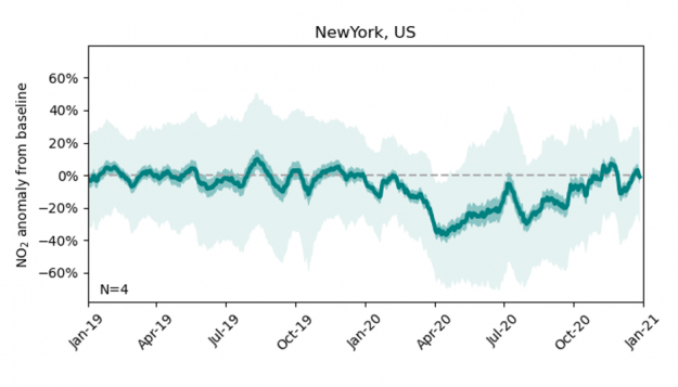
After training the XGBoost model on the 2018 and 2019 data (using 8-fold cross-validation), we extend the NO2 bias correction to the model data produced for year 2020, resulting in a time series of the expected NO2 concentrations at a given observation site if there had been no mobility restrictions due to the pandemic (the NO2 ‘baseline’). The difference between the actual observations and these bias-corrected model predictions offers an estimate of the impact of COVID-19 restrictions on NO2 concentrations. The figure below shows the difference between observations and model predictions at New York City from Jan 2019 to Jan 2021. The solid green line shows the best estimate, defined as the 21-day rolling average across all four observation sites available for New York City, and the dark and light shaded areas show two uncertainty estimates derived from the time-averaged and hourly model-observation samples, respectively.
Throughout year 2019, the bias-corrected model mean estimate is in close agreement with the observations. Coinciding with the outbreak of the pandemic, the observed NO2 over New York City declines by up to 40% and only gradually recovers to the expected value by year end.
Figure 3: Dark and light-shaded areas indicate low and high uncertainty estimates.
Conducting this analysis at 4,778 locations across the world enables us to identify regional patterns in air quality anomalies, and our study shows that these patterns tend to be related to differences in timing and intensity of COVID-19 restrictions.
The here described approach is not only useful to analyze the impact of COVID-19 on air pollution but can be generally used to monitor air pollution across the world (both the observations and model data are available in near real-time). Given the growing number of available air quality observations, fast data processing becomes ever more critical for such an application. The sample code available at https://github.com/GEOS-CF/covid_no2 demonstrates that conducting the analysis on a V100 GPU using cuDF offers an overall speed-up of up to 5x for, each city compared to 20-core Intel Xeon E5-2689 CPU.
References:
Keller, C. A., Evans, M. J., Knowland, K. E., Hasenkopf, C. A., Modekurty, S., Lucchesi, R. A., Oda, T., Franca, B. B., Mandarino, F. C., Díaz Suárez, M. V., Ryan, R. G., Fakes, L. H., and Pawson, S.: Global impact of COVID-19 restrictions on the surface concentrations of nitrogen dioxide and ozone, Atmos. Chem. Phys., 21, 3555–3592, https://doi.org/10.5194/acp-21-3555-2021, 2021.
I’m trying to use Tensorflow to predict the outcome of a sport contest. What I have for every sample is the context of the competition (weather, type of stadium, …) and the competition history for every competing team.
Here is an overview of the data of every sample:
Context
Teams History
CompetitionData
[[CompetitionData], [CompetitionData]] (for every team, the past competition data and their result (win/lose/ranking)
I’m going to try to develop a Learning to Rank System, where given the context and every team history, predict the final ranking.
I think that feature columns are useful in this case, as they can ease the processing of the Competition Data. However, I can’t find a way to reuse the feature column code across all Competition data dimensions. The ideal would be to reuse the DenseFeatures layers across all competition data, but it doesn’t seems to work as tf requires the data to be of dict type to be fed to the Densefeature layers, which needs to be passed one by one trough an input layer to be correctly inputted.
statics_hist = {
‘rapport’: Input((1,), dtype=tf.dtypes.int32, name=”rapport”),
‘weight’: Input((1,), dtype=tf.dtypes.int32, name=”weight”),
‘age’: Input((1,), name=”age”),
‘first’: Input((1,), dtype=tf.dtypes.int32, name=”first”),
‘stadium’: Input((1,), name=”stadiul”, dtype=tf.dtypes.string)
}
test = [stack([history_input(statics_hist) for _ in range(NB_RACE_HISTORY)], axis=1) for __ in range(MAX_NUMBER_PLAYERS)]
test = stack(test, axis=1)
But as I have 15 players with each 10 competition history of several columns, this gives me 750+ input layers, which can’t be the right way to go.
I have thought about flattening the data beforehand, but then I would lose the ability to run an LSTM trough a player history, which is important to modelize his current performance.
I’m not really sure of the right way to go, could anyone point me in the right direction ?


 This year, everyone can learn how to develop safe, robust autonomous vehicles on NVIDIA DRIVE. The annual DRIVE Developer Days is taking place April 20-22 during GTC 2021, featuring a series of specialized sessions on autonomous vehicle hardware and software, including perception, mapping, simulation and more, all led by NVIDIA experts. And now, registration is …
 Over the past couple of years, NVIDIA and NASA have been working closely on accelerating data science workflows using RAPIDS, and integrating these GPU-accelerated libraries with scientific use cases. This is the second post in a series that will discuss the results from an air pollution monitoring use case conducted during the COVID-19 pandemic, and …