Category: Misc

In a previous post, I gave an introduction to Policy Gradient reinforcement learning. Policy gradient-based reinforcement learning relies on using neural networks to learn an action policy for the control of agents in an environment. This is opposed to controlling agents based on neural network estimations of a value-based function, such as the Q value in deep Q learning. However, there are problems with straight Monte-Carlo based methods of policy gradient learning as covered in the previously mentioned policy gradient post. In particular, one significant problem is a high variance in the learning. This problem can be solved by a process called baselining, with the most effective baselining method being the Advantage Actor Critic method or A2c. In this post, I’ll review the theory of the A2c method, and demonstrate how to build an A2c algorithm in TensorFlow 2.

All code shown in this tutorial can be found at this site’s Github repository, in the ac2_tf2_cartpole.py file.

A quick recap of some important concepts

In the A2C algorithm, notice the title “Advantage Actor” – this refers first to the actor, the part of the neural network that is used to determine the actions of the agent. The “advantage” is a concept that expresses the relative benefit of taking a certain action at time t ($a_t$) from a certain state $s_t$. Note that it is not the “absolute” benefit, but the “relative” benefit. This will become clearer when I discuss the concept of “value”. The advantage is expressed as:

$$A(s_t, a_t) = Q(s_t, a_t) – V(s_t)$$

The Q value (discussed in other posts, for instance here, here and here) is the expected future rewards of taking action $a_t$ from state $s_t$. The value $V(s_t)$ is the expected value of the agent being in that state and operating under a certain action policy $pi$. It can be expressed as:

$$V^{pi}(s) = mathbb{E} left[sum_{i=1}^T gamma^{i-1}r_{i}right]$$

Here $mathbb{E}$ is the expectation operator, and the value $V^{pi}(s)$ can be read as the expected value of future discounted rewards that will be gathered by the agent, operating under a certain action policy $pi$. So, the Q value is the expected value of taking a certain action from the current state, whereas V is the expected value of simply being in the current state, under a certain action policy.

The advantage then is the relative benefit of taking a certain action from the current state. It’s kind of like a normalized Q value. For example, let’s consider the last state in a game, where after the next action the game ends. There are three possible actions from this state, with rewards of (51, 50, 49). Let’s also assume that the action selection policy $pi$ is simply random, so there is an equal chance of any of the three actions being selected. The value of this state, then, is 50 ((51+50+49) / 3). If the first action is randomly selected (reward=51), the Q value is 51. However, the advantage is only equal to 1 (Q-V = 51-50). As can be observed and as stated above, the advantage is a kind of normalized or relative Q value.

Why is this important? If we are using Q values in some way to train our action-taking policy, in the example above the first action would send a “signal” or contribution of 51 to the gradient optimizer, which may be significant enough to push the parameters of the neural network significantly in a certain direction. However, given the other two actions possible from this state also have a high reward (50 and 49), the signal or contribution is really higher than it should be – it is not that much better to take action 1 instead of action 3. Therefore, Q values can be a source of high variance in the training process, and it is much better to use the normalized or baseline Q values i.e. the advantage, in training. For more discussion of Q, values, and advantages, see my post on dueling Q networks.

Policy gradient reinforcement learning and its problems

In a previous post, I presented the policy gradient reinforcement learning algorithm. For details on this algorithm, please consult that post. However, the A2C algorithm shares important similarities with the PG algorithm, and therefore it is necessary to recap some of the theory. First, it has to be recalled that PG-based algorithms involve a neural network that directly outputs estimates of the probability distribution of the best next action to take in a given state. So, for instance, if we have an environment with 4 possible actions, the output from the neural network could be something like [0.5, 0.25, 0.1, 0.15], with the first action being currently favored. In the PG case, then, the neural network is the direct instantiation of the policy of the agent $pi_{theta}$ – where this policy is controlled by the parameters of the neural network $theta$. This is opposed to Q based RL algorithms, where the neural network estimates the Q value in a given state for each possible action. In these algorithms, the action policy is generally an epsilon-greedy policy, where the best action is that action with the highest Q value (with some random choices involved to improve exploration).

The gradient of the loss function for the policy gradient algorithm is as follows:

$$nabla_theta J(theta) sim left(sum_{t=0}^{T-1} log P_{pi_{theta}}(a_t|s_t)right)left(sum_{t’= t + 1}^{T} gamma^{t’-t-1} r_{t’} right)$$

Note that the term:

$$G_t = left(sum_{t’= t + 1}^{T} gamma^{t’-t-1} r_{t’} right)$$

Is just the discounted sum of the rewards onwards from state $s_t$. In other words, it is an estimate of the true value function $V^{pi}(s)$. Remember that in the PG algorithm, the network can only be trained after each full episode, and this is because of the term above. Therefore, note that the $G_t$ term above is an estimate of the true value function as it is based on only a single trajectory of the agent through the game.

Now, because it is based on samples of reward trajectories, which aren’t “normalized” or baselined in any way, the PG algorithm suffers from variance issues, resulting in slower and more erratic training progress. A better solution is to replace the $G_t$ function above with the Advantage – $A(s_t, a_t)$, and this is what the Advantage-Actor Critic method does.

The A2C algorithm

Replacing the $G_t$ function with the advantage, we come up with the following gradient function which can be used in training the neural network:

$$nabla_theta J(theta) sim left(sum_{t=0}^{T-1} log P_{pi_{theta}}(a_t|s_t)right)A(s_t, a_t)$$

Now, as shown above, the advantage is:

$$A(s_t, a_t) = Q(s_t, a_t) – V(s_t)$$

However, using Bellman’s equation, the Q value can be expressed purely in terms of the rewards and the value function:

$$Q(s_t, a_t) = mathbb{E}left[r_{t+1} + gamma V(s_{t+1})right]$$

Therefore, the advantage can now be estimated as:

$$A(s_t, a_t) = r_{t+1} + gamma V(s_{t+1}) – V(s_t)$$

As can be seen from the above, there is a requirement to be able to estimate the value function V. We could estimate it by running our agents through full episodes, in the same way we did in the policy gradient method. However, it would be better to be able to just collect batches of game-steps and train whenever the batch buffer was full, rather than having to wait for an episode to finish. That way, the agent could actually learn “on-the-go” during the middle of an episode/game.

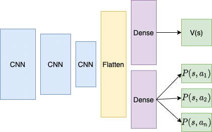
So, do we build another neural network to estimate V? We could have two networks, one to learn the policy and produce actions, and another to estimate the state values. A more efficient solution is to create one network, but with two output channels, and this is how the A2C method is outworked. The figure below shows the network architecture for an A2C neural network:

A2C architecture

This architecture is based on an A2C method that takes game images as the state input, hence the convolutional neural network layers at the beginning of the network (for more on CNNs, see my post here). This network architecture also resembles the Dueling Q network architecture (see my Dueling Q post). The point to note about the architecture above is that most of the network is shared, with a late bifurcation between the policy part and the value part. The outputs $P(s, a_i)$ are the action probabilities of the policy (generated from the neural network) – $P(a_t|s_t)$. The other output channel is the value estimation – a scalar output which is the predicted value of state s – $V(s)$. The two dense channels disambiguate the policy and the value outputs from the front-end of the neural network.

In this example, we’ll just be demonstrating the A2C algorithm on the Cartpole OpenAI Gym environment which doesn’t require a visual state input (i.e. a set of pixels as the input to the NN), and therefore the two output channels will simply share some dense layers, rather than a series of CNN layers.

The A2C loss functions

There are actually three loss values that need to be calculated in the A2C algorithm. Each of these losses is in practice given a weighting, and then they are summed together (with the entropy loss having a negative sign, see below).

The Critic loss

The loss function of the Critic i.e. the value estimating output of the neural network $V(s)$, needs to be trained so that it predicts more and more closely the actual value of the state. As shown before, the value of a state is calculated as:

$$V^{pi}(s) = mathbb{E} left[sum_{i=1}^T gamma^{i-1}r_{i}right]$$

So $V^{pi}(s)$ is the expected value of the discounted future rewards obtained by outworking a trajectory through the game based on a certain operating policy $pi$. We can therefore compare the predicted $V(s)$ at each state in the game, and the actual sampled discounted rewards that were gathered, and the difference between the two is the Critic loss. In this example, we’ll use a mean squared error function as the loss function, between the discounted rewards and the predicted values ($(V(s) – DR)^2$).

Now, given that, under the A2C algorithm, we collect state, action and reward tuples until a batch buffer is filled, how are we meant to figure out this discounted rewards sum? Let’s say we progress 3 states through a game, and we collect:

$(V(s_0), r_0), (V(s_1), r_1), (V(s_2), r_2)$

For the first Critic loss, we could calculate it as:

$$MSE(V(s_0), r_0 + gamma r_1 + gamma^2 r_2)$$

But that is missing all the following rewards $r_3, r_4, …., r_n$ until the game terminates. We didn’t have this problem in the Policy Gradient method, because in that method, we made sure a full run through the game had completed before training the neural network. In the A2c method, we use a trick called bootstrapping. To replace all the discounted $r_3, r_4, …., r_n$ values, we get the network to estimate the value for state 3, $V(s_3)$, and this will be an estimate for all the discounted future rewards beyond that point in the game. So, for the first Critic loss, we would have:

$$MSE(V(s_0), r_0 + gamma r_1 + gamma^2 r_2 + gamma^3 V(s_3))$$

Where $V(s_3)$ is a bootstrapped estimate of the value of the next state $s_3$.

This will be explained more in the code-walkthrough to follow.

The Actor loss

The second loss function needs to train the Actor (i.e. the action policy). Recall that the advantage weighted policy loss is:

$$nabla_theta J(theta) sim left(sum_{t=0}^{T-1} log P_{pi_{theta}}(a_t|s_t)right)A(s_t, a_t)$$

Let’s start with the advantage – $A(s_t, a_t) = r_{t+1} + gamma V(s_{t+1}) – V(s_t)$

This is simply the bootstrapped discounted rewards minus the predicted state values $V(s_t)$ that we gathered up while playing the game. So calculating the advantage is quite straight-forward, once we have the bootstrapped discounted rewards, as will be seen in the code walk-through shortly.

Now, with regards to the $log P_{pi_{theta}}(a_t|s_t)$ statement, in this instance, we can just calculate the log of the softmax probability estimate for whatever action was taken. So, for instance, if in state 1 ($s_1$) the network softmax output produces {0.1, 0.9} (for a 2-action environment), and the second action was actually taken by the agent, we would want to calculate log(0.9). We can make use of the TensorFlow-Keras SparseCategoricalCrossEntropy calculation, which takes the action as an integer, and this specifies which softmax output value to apply the log to. So in this example, y_pred = [1] and y_target = [0.1, 0.9] and the answer would be -log(0.9) = 0.105.

Another handy feature with the SpareCategoricalCrossEntropy loss in Keras is that it can be called with a “sample_weight” argument. This basically multiplies the log calculation with a value. So, in this example, we can supply the advantages as the sample weights, and it will calculate  $nabla_theta J(theta) sim left(sum_{t=0}^{T-1} log P_{pi_{theta}}(a_t|s_t)right)A(s_t, a_t)$ for us. This will be shown below, but the call will look like:

policy_loss = sparse_ce(actions, policy_logits, sample_weight=advantages)

Entropy loss

In many implementations of the A2c algorithm, another loss term is subtracted – the entropy loss. Entropy is a measure, broadly speaking, of randomness. The higher the entropy, the more random the state of affairs, the lower the entropy, the more ordered the state of affairs. In the case of A2c, entropy is calculated on the softmax policy action ($P(a_t|s_t)$) output of the neural network. Let’s go back to our two action example from above. In the case of a probability output of {0.1, 0.9} for the two possible actions, this is an ordered, less-random selection of actions. In other words, there will be a consistent selection of action 2, and only rarely will action 1 be taken. The entropy formula is:

$$E = -sum p(x) log(p(x))$$

So in this case, the entropy of that output would be 0.325. However, if the probability output was instead {0.5, 0.5}, the entropy would be 0.693. The 50-50 action probability distribution will produce more random actions, and therefore the entropy is higher.

By subtracting the entropy calculation from the total loss (or giving the entropy loss a negative sign), it encourages more randomness and therefore more exploration. The A2c algorithm can have a tendency of converging on particular actions, so this subtraction of the entropy encourages a better exploration of alternative actions, though making the weighting on this component of the loss too large can also reduce training performance.

Again, we can use an already existing Keras loss function to calculate the entropy. The Keras categorical cross-entropy performs the following calculation:

Keras output of cross-entropy loss function

If we just pass in the probability outputs as both target and output to this function, then it will calculate the entropy for us. This will be shown in the code below.

The total loss

The total loss function for the A2C algorithm is:

Loss = Actor Loss + Critic Loss * CRITIC_WEIGHT – Entropy Loss * ENTROPY_WEIGHT

A common value for the critic weight is 0.5, and the entropy weight is usually quite low (i.e. on the order of 0.01-0.001), though these hyperparameters can be adjusted and experimented with depending on the environment and network.

Implementing A2C in TensorFlow 2

In the following section, I will provide a walk-through of some code to implement the A2C methodology in TensorFlow 2. The code for this can be found at this site’s Github repository, in the ac2_tf2_cartpole.py file.

First, we perform the usual imports, set some constants, initialize the environment and finally create the neural network model which instantiates the A2C architecture:

import tensorflow as tf
from tensorflow import keras
import numpy as np
import gym
import datetime as dt

STORE_PATH = '/Users/andrewthomas/Adventures in ML/TensorFlowBook/TensorBoard/A2CCartPole'
CRITIC_LOSS_WEIGHT = 0.5
ACTOR_LOSS_WEIGHT = 1.0
ENTROPY_LOSS_WEIGHT = 0.05
BATCH_SIZE = 64
GAMMA = 0.95

env = gym.make("CartPole-v0")
state_size = 4
num_actions = env.action_space.n


class Model(keras.Model):
    def __init__(self, num_actions):
        super().__init__()
        self.num_actions = num_actions
        self.dense1 = keras.layers.Dense(64, activation='relu',
                                         kernel_initializer=keras.initializers.he_normal())
        self.dense2 = keras.layers.Dense(64, activation='relu',
                                         kernel_initializer=keras.initializers.he_normal())
        self.value = keras.layers.Dense(1)
        self.policy_logits = keras.layers.Dense(num_actions)

    def call(self, inputs):
        x = self.dense1(inputs)
        x = self.dense2(x)
        return self.value(x), self.policy_logits(x)

    def action_value(self, state):
        value, logits = self.predict_on_batch(state)
        action = tf.random.categorical(logits, 1)[0]
        return action, value

As can be seen, for this example I have set the critic, actor and entropy loss weights to 0.5, 1.0 and 0.05 respectively. Next the environment is setup, and then the model class is created.

This class inherits from keras.Model, which enables it to be integrated into the streamlined Keras methods of training and evaluating (for more information, see this Keras tutorial). In the initialization of the class, we see that 2 dense layers have been created, with 64 nodes in each. Then a value layer with one output is created, which evaluates $V(s)$, and finally the policy layer output with a size equal to the number of available actions. Note that this layer produces logits only, the softmax function which creates pseudo-probabilities ($P(a_t, s_t)$) will be applied within the various TensorFlow functions, as will be seen.

Next, the call function is defined – this function is run whenever a state needs to be “run” through the model, to produce a value and policy logits output. The Keras model API will use this function in its predict functions and also its training functions. In this function, it can be observed that the input is passed through the two common dense layers, and then the function returns first the value output, then the policy logits output.

The next function is the action_value function. This function is called upon when an action needs to be chosen from the model. As can be seen, the first step of the function is to run the predict_on_batch Keras model API function. This function just runs the model.call function defined above. The output is both the values and the policy logits. An action is then selected by randomly choosing an action based on the action probabilities. Note that tf.random.categorical takes as input logits, not softmax outputs. The next function, outside of the Model class, is the function that calculates the critic loss:

def critic_loss(discounted_rewards, predicted_values):
    return keras.losses.mean_squared_error(discounted_rewards, predicted_values) * CRITIC_LOSS_WEIGHT

As explained above, the critic loss comprises of the mean squared error between the discounted rewards (which is calculated in another function, soon to be discussed) and the values predicted from the value output of the model (which are accumulated in a list during the agent’s trajectory through the game).

The following function shows the actor loss function:

def actor_loss(combined, policy_logits):
    actions = combined[:, 0]
    advantages = combined[:, 1]
    sparse_ce = keras.losses.SparseCategoricalCrossentropy(
        from_logits=True, reduction=tf.keras.losses.Reduction.SUM
    )

    actions = tf.cast(actions, tf.int32)
    policy_loss = sparse_ce(actions, policy_logits, sample_weight=advantages)

    probs = tf.nn.softmax(policy_logits)
    entropy_loss = keras.losses.categorical_crossentropy(probs, probs)

    return policy_loss * ACTOR_LOSS_WEIGHT - entropy_loss * ENTROPY_LOSS_WEIGHT

The first argument to the actor_loss function is an array with two columns (and BATCH_SIZE rows). The first column corresponds to the recorded actions of the agent as it traversed the game. The second column is the calculated advantages – the calculation of which will be shown shortly. Next, the sparse categorical cross-entropy function class is created. The arguments specify that the input to the function is logits (i.e. they don’t have softmax applied to them yet), and it also specifies the reduction to apply to the BATCH_SIZE number of calculated losses – in this case, a sum() function which aligns with the summation in:

$$nabla_theta J(theta) sim left(sum_{t=0}^{T-1} log P_{pi_{theta}}(a_t|s_t)right)A(s_t, a_t)$$

Next, the actions are cast to be integers (rather than floats) and finally, the policy loss is calculated based on the sparse_ce function. As discussed above, the sparse categorical cross-entropy function will select those policy probabilities that correspond to the actions actually taken in the game, and weight them by the advantage values. By applying a summation reduction, the formula above will be implemented in this function.

Next, the actual probabilities for action are estimated by applying the softmax function to the logits, and the entropy loss is calculated by applying the categorical cross-entropy function. See the previous discussion on how this works.

The following function calculates the discounted reward values and the advantages:

def discounted_rewards_advantages(rewards, dones, values, next_value):
    discounted_rewards = np.array(rewards + [next_value[0]])

    for t in reversed(range(len(rewards))):
        discounted_rewards[t] = rewards[t] + GAMMA * discounted_rewards[t+1] * (1-dones[t])
    discounted_rewards = discounted_rewards[:-1]
    # advantages are bootstrapped discounted rewards - values, using Bellman's equation
    advantages = discounted_rewards - np.stack(values)[:, 0]
    return discounted_rewards, advantages

The first input value to this function is a list of all the rewards that were accumulated..

spectrogram_ds = waveform_ds.map(get_spectrogram_and_label_id, num_parallel_calls=AUTOTUNE) 

def get_spectrogram(waveform): # Padding for files with less than 16000 samples zero_padding = tf.zeros([16000] - tf.shape(waveform), dtype=tf.float32) # Concatenate audio with padding so that all audio clips will be of the # same length waveform = tf.cast(waveform, tf.float32) equal_length = tf.concat([waveform, zero_padding], 0) equal_length = equal_length.eval() # <-- HERE IS THE PROBLEM spectrogram = do_stft(equal_length, 512, 128) #<-- uses NUMPY return spectrogram def get_spectrogram_and_label_id(audio, label): print(sess.graph) spectrogram = get_spectrogram(audio.eval(session=sess)) spectrogram = tf.expand_dims(spectrogram, -1) label_id = tf.argmax(label == commands) return spectrogram, label_id spectrogram_ds = waveform_ds.map(get_spectrogram_and_label_id, num_parallel_calls=AUTOTUNE) 

submitted by /u/alex_bababu
[visit reddit] [comments]