|
submitted by /u/MLtinkerer [visit reddit] [comments] |
 DataBloom
|
|
submitted by /u/MLtinkerer [visit reddit] [comments] |
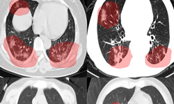
NVIDIA Inception partner DarwinAI developed a new AI model to detect COVID-19 in CT scans with 96% accuracy across a wide and diverse number of scenarios. The model, COVID-Net CT-2, was built using a number of large and diverse datasets created over several months with the University of Waterloo and is publicly available on GitHub.
Last year, the startup launched an open source neural network for COVID-19 detection called COVID-Net. Their new model builds upon the initiative with a more robust model, trained on the largest quantity and diversity of multinational patient cases in research literature. Their academic study detailing the construction and validation of the model can be found here.
DarwinAI used an NVIDIA RTX 6000 for training their neural network and the NVIDIA Jetson Nano embedded AI platform to run their inference workloads.
“By building COVID-NET CT-2 from such rich and voluminous data, we’ve been able to achieve a new level of screening accuracy, with COVID-19 sensitivity and positive predictive value exceeding 96% across a wide and diverse number of scenarios,” said Sheldon Fernandez, CEO of Darwin-AI.
“Our XAI platform was instrumental in the construction of the original COVID-Net model. For this version, we have engaged two senior radiologists in Canada to validate the way in which COVID-Net CT-2 makes its decisions. Much to our delight, both confirmed the decision-making process of COVID-Net CT-2 is consistent with their own expert interpretations,” Fernandez added. “In addition to illustrating the emerging cooperation between our respective domains, their validation exemplifies the importance of our XAI technology in constructing transparent and trustworthy AI.”

Both DarwinAI and NVIDIA are enabling researchers to build neural networks to fight COVID-19 with the help of open source AI and publicly available pre-trained models. Medical imaging AI models for detecting COVID-19 in X-rays and CTs can be accessed through DarwinAI’s COVID-Net Initiative and the NVIDIA COVID-19 NGC Catalog.
Learn more about how AI, accelerated computing, and GPU technology are contributing to the worldwide battle against the novel coronavirus in the COVID-19 Research Hub.
For many, the term “autonomous vehicles” conjures up images of self-driving cars. Autonomy, however, is transforming much more than personal transportation. Autonomous trucks are commercial vehicles that use AI to automate everything from shipping yard operations to long-haul deliveries. Due to industry pressures from rising delivery demand and driver shortages, as well as straightforward operational Read article >
The post The Truck Stops Here: How AI Is Creating a New Kind of Commercial Vehicle appeared first on The Official NVIDIA Blog.
It’s a celebration, gamers! One year ago to the day we launched GeForce NOW, our cloud gaming service that transforms ordinary hardware into an extraordinarily powerful GeForce gaming PC. It’s the always-on gaming rig that never needs upgrading or patching and can instantly play your library of games. We’ve been blown away by the passion Read article >
The post Achievement Unlocked: Celebrating Year One of GeForce NOW appeared first on The Official NVIDIA Blog.
Scientifically speaking, today is the best day of the week, because today is GFN Thursday. And that means more of the best PC games streaming right from the cloud across all of your devices. This is a special GFN Thursday, too — not just because it’s the first Thursday of the month, which means learning Read article >
The post GFN Thursday — 30 Games Coming in February, 13 Available Today appeared first on The Official NVIDIA Blog.

This article translates Daniel Falbel’s ‘Simple Audio Classification’ article from tensorflow/keras to torch/torchaudio. The main goal is to introduce torchaudio and illustrate its contributions to the torch ecosystem. Here, we focus on a popular dataset, the audio loader and the spectrogram transformer. An interesting side product is the parallel between torch and tensorflow, showing sometimes the differences, sometimes the similarities between them.
library(torch)
library(torchaudio)
Downloading and Importing
torchaudio has the speechcommand_dataset built in. It filters out background_noise by default and lets us choose between versions v0.01 and v0.02.
# set an existing folder here to cache the dataset
DATASETS_PATH <- "~/datasets/"

# 1.4GB download
df <- speechcommand_dataset(
  root = DATASETS_PATH,
  url = "speech_commands_v0.01",
  download = TRUE
)

# expect folder: _background_noise_
df$EXCEPT_FOLDER
# [1] "_background_noise_"

# number of audio files
length(df)
# [1] 64721

# a sample
sample <- df[1]

sample$waveform[, 1:10]
torch_tensor
0.0001 *
 0.9155  0.3052  1.8311  1.8311 -0.3052  0.3052  2.4414  0.9155 -0.9155 -0.6104
[ CPUFloatType{1,10} ]
sample$sample_rate
# 16000
sample$label
# bed

plot(sample$waveform[1], type = "l", col = "royalblue", main = sample$label)

(#fig:unnamed-chunk-4)A sample waveform for a ‘bed’.
Classes
df$classes
 [1] "bed"    "bird"   "cat"    "dog"    "down"   "eight"  "five"
 [8] "four"   "go"     "happy"  "house"  "left"   "marvin" "nine"
[15] "no"     "off"    "on"     "one"    "right"  "seven"  "sheila"
[22] "six"    "stop"   "three"  "tree"   "two"    "up"     "wow"
[29] "yes"    "zero"
Generator Dataloader
torch::dataloader has the same task as data_generator defined in the original article. It is responsible for preparing batches – including shuffling, padding, one-hot encoding, etc. – and for taking care of parallelism / device I/O orchestration.
In torch we do this by passing the train/test subset to torch::dataloader and encapsulating all the batch setup logic inside a collate_fn() function.
set.seed(6)
id_train <- sample(length(df), size = 0.7*length(df))
id_test <- setdiff(seq_len(length(df)), id_train)
# subsets

train_subset <- torch::dataset_subset(df, id_train)
test_subset <- torch::dataset_subset(df, id_test)
At this point, dataloader(train_subset) would not work because the samples are not padded. So we need to build our own collate_fn() with the padding strategy.
I suggest using the following approach when implementing the collate_fn():
collate_fn <- function(batch) {
  browser()
}

ds_train <- dataloader(
  train_subset,
  batch_size = 32,
  shuffle = TRUE,
  collate_fn = collate_fn
)

ds_train_env <- enumerate(ds_train)
ds_train_env[[1]][[1]]
The final collate_fn() pads the waveform to length 16001 and then stacks everything up together. At this point there are no spectrograms yet. We going to make spectrogram transformation a part of model architecture.
pad_sequence <- function(batch) {
    # Make all tensors in a batch the same length by padding with zeros
    batch <- sapply(batch, function(x) (x$t()))
    batch <- torch::nn_utils_rnn_pad_sequence(batch, batch_first = TRUE, padding_value = 0.)
    return(batch$permute(c(1, 3, 2)))
  }

# Final collate_fn
collate_fn <- function(batch) {
 # Input structure:
 # list of 32 lists: list(waveform, sample_rate, label, speaker_id, utterance_number)
 # Transpose it
 batch <- purrr::transpose(batch)
 tensors <- batch$waveform
 targets <- batch$label_index

 # Group the list of tensors into a batched tensor
 tensors <- pad_sequence(tensors)

 # target encoding
 targets <- torch::torch_stack(targets)

 list(tensors = tensors, targets = targets) # (64, 1, 16001)
}
Batch structure is:
Also, torchaudio comes with 3 loaders, av_loader, tuner_loader, and audiofile_loader- more to come. set_audio_backend() is used to set one of them as the audio loader. Their performances differ based on audio format (mp3 or wav). There is no perfect world yet: tuner_loader is best for mp3, audiofile_loader is best for wav, but neither of them has the option of partially loading a sample from an audio file without bringing all the data into memory first.
For a given audio backend we need pass it to each worker through worker_init_fn() argument.
ds_train <- dataloader(
  train_subset,
  batch_size = 128,
  shuffle = TRUE,
  collate_fn = collate_fn,
  num_workers = 16,
  worker_init_fn = function(.) {torchaudio::set_audio_backend("audiofile_loader")},
  worker_globals = c("pad_sequence") # pad_sequence is needed for collect_fn
)

ds_test <- dataloader(
  test_subset,
  batch_size = 64,
  shuffle = FALSE,
  collate_fn = collate_fn,
  num_workers = 8,
  worker_globals = c("pad_sequence") # pad_sequence is needed for collect_fn
)
Model definition
Instead of keras::keras_model_sequential(), we are going to define a torch::nn_module(). As referenced by the original article, the model is based on this architecture for MNIST from this tutorial, and I’ll call it ‘DanielNN’.
dan_nn <- torch::nn_module(
  "DanielNN",

  initialize = function(
    window_size_ms = 30,
    window_stride_ms = 10
  ) {

    # spectrogram spec
    window_size <- as.integer(16000*window_size_ms/1000)
    stride <- as.integer(16000*window_stride_ms/1000)
    fft_size <- as.integer(2^trunc(log(window_size, 2) + 1))
    n_chunks <- length(seq(0, 16000, stride))

    self$spectrogram <- torchaudio::transform_spectrogram(
      n_fft = fft_size,
      win_length = window_size,
      hop_length = stride,
      normalized = TRUE,
      power = 2
    )

    # convs 2D
    self$conv1 <- torch::nn_conv2d(in_channels = 1, out_channels = 32, kernel_size = c(3,3))
    self$conv2 <- torch::nn_conv2d(in_channels = 32, out_channels = 64, kernel_size = c(3,3))
    self$conv3 <- torch::nn_conv2d(in_channels = 64, out_channels = 128, kernel_size = c(3,3))
    self$conv4 <- torch::nn_conv2d(in_channels = 128, out_channels = 256, kernel_size = c(3,3))

    # denses
    self$dense1 <- torch::nn_linear(in_features = 14336, out_features = 128)
    self$dense2 <- torch::nn_linear(in_features = 128, out_features = 30)
  },

  forward = function(x) {
    x %>% # (64, 1, 16001)
      self$spectrogram() %>% # (64, 1, 257, 101)
      torch::torch_add(0.01) %>%
      torch::torch_log() %>%
      self$conv1() %>%
      torch::nnf_relu() %>%
      torch::nnf_max_pool2d(kernel_size = c(2,2)) %>%

      self$conv2() %>%
      torch::nnf_relu() %>%
      torch::nnf_max_pool2d(kernel_size = c(2,2)) %>%

      self$conv3() %>%
      torch::nnf_relu() %>%
      torch::nnf_max_pool2d(kernel_size = c(2,2)) %>%

      self$conv4() %>%
      torch::nnf_relu() %>%
      torch::nnf_max_pool2d(kernel_size = c(2,2)) %>%

      torch::nnf_dropout(p = 0.25) %>%
      torch::torch_flatten(start_dim = 2) %>%

      self$dense1() %>%
      torch::nnf_relu() %>%
      torch::nnf_dropout(p = 0.5) %>%
      self$dense2()
  }
)

model <- dan_nn()


device <- torch::torch_device(if(torch::cuda_is_available()) "cuda" else "cpu")
model$to(device = device)

print(model)
An `nn_module` containing 2,226,846 parameters.

── Modules ──────────────────────────────────────────────────────
● spectrogram: <Spectrogram> #0 parameters
● conv1: <nn_conv2d> #320 parameters
● conv2: <nn_conv2d> #18,496 parameters
● conv3: <nn_conv2d> #73,856 parameters
● conv4: <nn_conv2d> #295,168 parameters
● dense1: <nn_linear> #1,835,136 parameters
● dense2: <nn_linear> #3,870 parameters
Model fitting
Unlike in tensorflow, there is no model %>% compile(…) step in torch, so we are going to set loss criterion, optimizer strategy and evaluation metrics explicitly in the training loop.
loss_criterion <- torch::nn_cross_entropy_loss()
optimizer <- torch::optim_adadelta(model$parameters, rho = 0.95, eps = 1e-7)
metrics <- list(acc = yardstick::accuracy_vec)
Training loop
library(glue)
library(progress)

pred_to_r <- function(x) {
  classes <- factor(df$classes)
  classes[as.numeric(x$to(device = "cpu"))]
}

set_progress_bar <- function(total) {
  progress_bar$new(
    total = total, clear = FALSE, width = 70,
    format = ":current/:total [:bar] - :elapsed - loss: :loss - acc: :acc"
  )
}
epochs <- 20
losses <- c()
accs <- c()

for(epoch in seq_len(epochs)) {
  pb <- set_progress_bar(length(ds_train))
  pb$message(glue("Epoch {epoch}/{epochs}"))
  coro::loop(for(batch in ds_train) {
    optimizer$zero_grad()
    predictions <- model(batch[[1]]$to(device = device))
    targets <- batch[[2]]$to(device = device)
    loss <- loss_criterion(predictions, targets)
    loss$backward()
    optimizer$step()

    # eval reports
    prediction_r <- pred_to_r(predictions$argmax(dim = 2))
    targets_r <- pred_to_r(targets)
    acc <- metrics$acc(targets_r, prediction_r)
    accs <- c(accs, acc)
    loss_r <- as.numeric(loss$item())
    losses <- c(losses, loss_r)

    pb$tick(tokens = list(loss = round(mean(losses), 4), acc = round(mean(accs), 4)))
  })
}


# test
predictions_r <- c()
targets_r <- c()
coro::loop(for(batch_test in ds_test) {
  predictions <- model(batch_test[[1]]$to(device = device))
  targets <- batch_test[[2]]$to(device = device)
  predictions_r <- c(predictions_r, pred_to_r(predictions$argmax(dim = 2)))
  targets_r <- c(targets_r, pred_to_r(targets))
})
val_acc <- metrics$acc(factor(targets_r, levels = 1:30), factor(predictions_r, levels = 1:30))
cat(glue("val_acc: {val_acc}nn"))
Epoch 1/20
[W SpectralOps.cpp:590] Warning: The function torch.rfft is deprecated and will be removed in a future PyTorch release. Use the new torch.fft module functions, instead, by importing torch.fft and calling torch.fft.fft or torch.fft.rfft. (function operator())
354/354 [=========================] -  1m - loss: 2.6102 - acc: 0.2333
Epoch 2/20
354/354 [=========================] -  1m - loss: 1.9779 - acc: 0.4138
Epoch 3/20
354/354 [============================] -  1m - loss: 1.62 - acc: 0.519
Epoch 4/20
354/354 [=========================] -  1m - loss: 1.3926 - acc: 0.5859
Epoch 5/20
354/354 [==========================] -  1m - loss: 1.2334 - acc: 0.633
Epoch 6/20
354/354 [=========================] -  1m - loss: 1.1135 - acc: 0.6685
Epoch 7/20
354/354 [=========================] -  1m - loss: 1.0199 - acc: 0.6961
Epoch 8/20
354/354 [=========================] -  1m - loss: 0.9444 - acc: 0.7181
Epoch 9/20
354/354 [=========================] -  1m - loss: 0.8816 - acc: 0.7365
Epoch 10/20
354/354 [=========================] -  1m - loss: 0.8278 - acc: 0.7524
Epoch 11/20
354/354 [=========================] -  1m - loss: 0.7818 - acc: 0.7659
Epoch 12/20
354/354 [=========================] -  1m - loss: 0.7413 - acc: 0.7778
Epoch 13/20
354/354 [=========================] -  1m - loss: 0.7064 - acc: 0.7881
Epoch 14/20
354/354 [=========================] -  1m - loss: 0.6751 - acc: 0.7974
Epoch 15/20
354/354 [=========================] -  1m - loss: 0.6469 - acc: 0.8058
Epoch 16/20
354/354 [=========================] -  1m - loss: 0.6216 - acc: 0.8133
Epoch 17/20
354/354 [=========================] -  1m - loss: 0.5985 - acc: 0.8202
Epoch 18/20
354/354 [=========================] -  1m - loss: 0.5774 - acc: 0.8263
Epoch 19/20
354/354 [==========================] -  1m - loss: 0.5582 - acc: 0.832
Epoch 20/20
354/354 [=========================] -  1m - loss: 0.5403 - acc: 0.8374
val_acc: 0.876705979296493
Making predictions
We already have all predictions calculated for test_subset, let’s recreate the alluvial plot from the original article.
library(dplyr)
library(alluvial)
df_validation <- data.frame(
  pred_class = df$classes[predictions_r],
  class = df$classes[targets_r]
)
x <-  df_validation %>%
  mutate(correct = pred_class == class) %>%
  count(pred_class, class, correct)

alluvial(
  x %>% select(class, pred_class),
  freq = x$n,
  col = ifelse(x$correct, "lightblue", "red"),
  border = ifelse(x$correct, "lightblue", "red"),
  alpha = 0.6,
  hide = x$n < 20
)
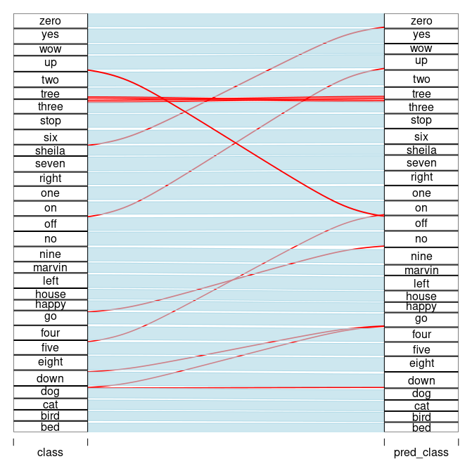
(#fig:unnamed-chunk-15)Model performance: true labels <–> predicted labels.
Model accuracy is 87,7%, somewhat worse than tensorflow version from the original post. Nevertheless, all conclusions from original post still hold.

submitted by /u/MLtinkerer
[visit reddit] [comments]
|
submitted by /u/MLtinkerer [visit reddit] [comments] |
submitted by /u/ashmortar
[visit reddit] [comments]
For my thesis, I am attempting to detect faults/inconsistencies in 3D prints.
Generating data takes a long time (because the print process takes a long time). For this reason my dataset is limited. I’ve got two classes which each have about 100-150 images each. This adds up to a total of about 250-300 images.Then I augmented those images 8 times with rotations and flips. I first tried to train on EfficientdetD0 but the results were pretty disappointing. Perhaps only a quarter of errors were getting detected.
Someone on this subreddit told me I should use an architecture like ” SSD ResNet50 V1 FPN 640×640 (RetinaNet50) ” because this appearantly works better for small datasets, though I don’t know why. So I went and tried it. I trained with the same parameters as before and for roughly the same time. The results were even worse.
Right now I would like to train a model from scratch and compare the results to the results I got using transfer learning, however I have no clue on how I should get started with this. I’ve been googling about but I haven’t found a clear explanation just yet. Could somebody please point me in the right direction?
Also why should SSD ResNet50 V1 FPN 640×640 (RetinaNet50) work better with smaller datasets, and why shouldn’t I just use ResNet 151? From what I’ve gathered this should work better than 50 in my case because it goed deeper, no?
submitted by /u/007Nick700
[visit reddit] [comments]