Categories
Offsites

Why π is in the normal distribution (beyond integral tricks)

Categories
Offsites

But what is the Central Limit Theorem?

Categories
Offsites

Barkour: Benchmarking animal-level agility with quadruped robots

Creating robots that exhibit robust and dynamic locomotion capabilities, similar to animals or humans, has been a long-standing goal in the robotics community. In addition to completing tasks quickly and efficiently, agility allows legged robots to move through complex environments that are otherwise difficult to traverse. Researchers at Google have been pursuing agility for multiple years and across various form factors. Yet, while researchers have enabled robots to hike or jump over some obstacles, there is still no generally accepted benchmark that comprehensively measures robot agility or mobility. In contrast, benchmarks are driving forces behind the development of machine learning, such as ImageNet for computer vision, and OpenAI Gym for reinforcement learning (RL).

In “Barkour: Benchmarking Animal-level Agility with Quadruped Robots”, we introduce the Barkour agility benchmark for quadruped robots, along with a Transformer-based generalist locomotion policy. Inspired by dog agility competitions, a legged robot must sequentially display a variety of skills, including moving in different directions, traversing uneven terrains, and jumping over obstacles within a limited timeframe to successfully complete the benchmark. By providing a diverse and challenging obstacle course, the Barkour benchmark encourages researchers to develop locomotion controllers that move fast in a controllable and versatile way. Furthermore, by tying the performance metric to real dog performance, we provide an intuitive metric to understand the robot performance with respect to their animal counterparts.

We invited a handful of dooglers to try the obstacle course to ensure that our agility objectives were realistic and challenging. Small dogs complete the obstacle course in approximately 10s, whereas our robot’s typical performance hovers around 20s.

Barkour benchmark

The Barkour scoring system uses a per obstacle and an overall course target time based on the target speed of small dogs in the novice agility competitions (about 1.7m/s). Barkour scores range from 0 to 1, with 1 corresponding to the robot successfully traversing all the obstacles along the course within the allotted time of approximately 10 seconds, the average time needed for a similar-sized dog to traverse the course. The robot receives penalties for skipping, failing obstacles, or moving too slowly.

Our standard course consists of four unique obstacles in a 5m x 5m area. This is a denser and smaller setup than a typical dog competition to allow for easy deployment in a robotics lab. Beginning at the start table, the robot needs to weave through a set of poles, climb an A-frame, clear a 0.5m broad jump and then step onto the end table. We chose this subset of obstacles because they test a diverse set of skills while keeping the setup within a small footprint. As is the case for real dog agility competitions, the Barkour benchmark can be easily adapted to a larger course area and may incorporate a variable number of obstacles and course configurations.

Overview of the Barkour benchmark’s obstacle course setup, which consists of weave poles, an A-frame, a broad jump, and pause tables. The intuitive scoring mechanism, inspired by dog agility competitions, balances speed, agility and performance and can be easily modified to incorporate other types of obstacles or course configurations.

Learning agile locomotion skills

The Barkour benchmark features a diverse set of obstacles and a delayed reward system, which pose a significant challenge when training a single policy that can complete the entire obstacle course. So in order to set a strong performance baseline and demonstrate the effectiveness of the benchmark for robotic agility research, we adopt a student-teacher framework combined with a zero-shot sim-to-real approach. First, we train individual specialist locomotion skills (teacher) for different obstacles using on-policy RL methods. In particular, we leverage recent advances in large-scale parallel simulation to equip the robot with individual skills, including walking, slope climbing, and jumping policies.

Next, we train a single policy (student) that performs all the skills and transitions in between by using a student-teacher framework, based on the specialist skills we previously trained. We use simulation rollouts to create datasets of state-action pairs for each one of the specialist skills. This dataset is then distilled into a single Transformer-based generalist locomotion policy, which can handle various terrains and adjust the robot’s gait based on the perceived environment and the robot’s state.

During deployment, we pair the locomotion transformer policy that is capable of performing multiple skills with a navigation controller that provides velocity commands based on the robot’s position. Our trained policy controls the robot based on the robot’s surroundings represented as an elevation map, velocity commands, and on-board sensory information provided by the robot.

Deployment pipeline for the locomotion transformer architecture. At deployment time, a high-level navigation controller guides the real robot through the obstacle course by sending commands to the locomotion transformer policy.

Robustness and repeatability are difficult to achieve when we aim for peak performance and maximum speed. Sometimes, the robot might fail when overcoming an obstacle in an agile way. To handle failures we train a recovery policy that quickly gets the robot back on its feet, allowing it to continue the episode.

Evaluation

We evaluate the Transformer-based generalist locomotion policy using custom-built quadruped robots and show that by optimizing for the proposed benchmark, we obtain agile, robust, and versatile skills for our robot in the real world. We further provide analysis for various design choices in our system and their impact on the system performance.

Model of the custom-built robots used for evaluation.

We deploy both the specialist and generalist policies to hardware (zero-shot sim-to-real). The robot’s target trajectory is provided by a set of waypoints along the various obstacles. In the case of the specialist policies, we switch between specialist policies by using a hand-tuned policy switching mechanism that selects the most suitable policy given the robot’s position.

Typical performance of our agile locomotion policies on the Barkour benchmark. Our custom-built quadruped robot robustly navigates the terrain’s obstacles by leveraging various skills learned using RL in simulation.

We find that very often our policies can handle unexpected events or even hardware degradation resulting in good average performance, but failures are still possible. As illustrated in the image below, in case of failures, our recovery policy quickly gets the robot back on its feet, allowing it to continue the episode. By combining the recovery policy with a simple walk-back-to-start policy, we are able to run repeated experiments with minimal human intervention to measure the robustness.

Qualitative example of robustness and recovery behaviors. The robot trips and rolls over after heading down the A-frame. This triggers the recovery policy, which enables the robot to get back up and continue the course.

We find that across a large number of evaluations, the single generalist locomotion transformer policy and the specialist policies with the policy switching mechanism achieve similar performance. The locomotion transformer policy has a slightly lower average Barkour score, but exhibits smoother transitions between behaviors and gaits.

Measuring robustness of the different policies across a large number of runs on the Barkour benchmark.

Histogram of the agility scores for the locomotion transformer policy. The highest scores shown in blue (0.75 – 0.9) represent the runs where the robot successfully completes all obstacles.

Conclusion

We believe that developing a benchmark for legged robotics is an important first step in quantifying progress toward animal-level agility. To establish a strong baseline, we investigated a zero-shot sim-to-real approach, taking advantage of large-scale parallel simulation and recent advancements in training Transformer-based architectures. Our findings demonstrate that Barkour is a challenging benchmark that can be easily customized, and that our learning-based method for solving the benchmark provides a quadruped robot with a single low-level policy that can perform a variety of agile low-level skills.

Acknowledgments

The authors of this post are now part of Google DeepMind. We would like to thank our co-authors at Google DeepMind and our collaborators at Google Research: Wenhao Yu, J. Chase Kew, Tingnan Zhang, Daniel Freeman, Kuang-Hei Lee, Lisa Lee, Stefano Saliceti, Vincent Zhuang, Nathan Batchelor, Steven Bohez, Federico Casarini, Jose Enrique Chen, Omar Cortes, Erwin Coumans, Adil Dostmohamed, Gabriel Dulac-Arnold, Alejandro Escontrela, Erik Frey, Roland Hafner, Deepali Jain, Yuheng Kuang, Edward Lee, Linda Luu, Ofir Nachum, Ken Oslund, Jason Powell, Diego Reyes, Francesco Romano, Feresteh Sadeghi, Ron Sloat, Baruch Tabanpour, Daniel Zheng, Michael Neunert, Raia Hadsell, Nicolas Heess, Francesco Nori, Jeff Seto, Carolina Parada, Vikas Sindhwani, Vincent Vanhoucke, and Jie Tan. We would also like to thank Marissa Giustina, Ben Jyenis, Gus Kouretas, Nubby Lee, James Lubin, Sherry Moore, Thinh Nguyen, Krista Reymann, Satoshi Kataoka, Trish Blazina, and the members of the robotics team at Google DeepMind for their contributions to the project.Thanks to John Guilyard for creating the animations in this post.

Categories
Offsites

Differentially private clustering for large-scale datasets

Clustering is a central problem in unsupervised machine learning (ML) with many applications across domains in both industry and academic research more broadly. At its core, clustering consists of the following problem: given a set of data elements, the goal is to partition the data elements into groups such that similar objects are in the same group, while dissimilar objects are in different groups. This problem has been studied in math, computer science, operations research and statistics for more than 60 years in its myriad variants. Two common forms of clustering are metric clustering, in which the elements are points in a metric space, like in the k-means problem, and graph clustering, where the elements are nodes of a graph whose edges represent similarity among them.

In the k-means clustering problem, we are given a set of points in a metric space with the objective to identify k representative points, called centers (here depicted as triangles), so as to minimize the sum of the squared distances from each point to its closest center. Source, rights: CC-BY-SA-4.0

Despite the extensive literature on algorithm design for clustering, few practical works have focused on rigorously protecting the user’s privacy during clustering. When clustering is applied to personal data (e.g., the queries a user has made), it is necessary to consider the privacy implications of using a clustering solution in a real system and how much information the output solution reveals about the input data.

To ensure privacy in a rigorous sense, one solution is to develop differentially private (DP) clustering algorithms. These algorithms ensure that the output of the clustering does not reveal private information about a specific data element (e.g., whether a user has made a given query) or sensitive data about the input graph (e.g., a relationship in a social network). Given the importance of privacy protections in unsupervised machine learning, in recent years Google has invested in research on theory and practice of differentially private metric or graph clustering, and differential privacy in a variety of contexts, e.g., heatmaps or tools to design DP algorithms.

Today we are excited to announce two important updates: 1) a new differentially-private algorithm for hierarchical graph clustering, which we’ll be presenting at ICML 2023, and 2) the open-source release of the code of a scalable differentially-private k-means algorithm. This code brings differentially private k-means clustering to large scale datasets using distributed computing. Here, we will also discuss our work on clustering technology for a recent launch in the health domain for informing public health authorities.

Differentially private hierarchical clustering

Hierarchical clustering is a popular clustering approach that consists of recursively partitioning a dataset into clusters at an increasingly finer granularity. A well known example of hierarchical clustering is the phylogenetic tree in biology in which all life on Earth is partitioned into finer and finer groups (e.g., kingdom, phylum, class, order, etc.). A hierarchical clustering algorithm receives as input a graph representing the similarity of entities and learns such recursive partitions in an unsupervised way. Yet at the time of our research no algorithm was known to compute hierarchical clustering of a graph with edge privacy, i.e., preserving the privacy of the vertex interactions.

In “Differentially-Private Hierarchical Clustering with Provable Approximation Guarantees”, we consider how well the problem can be approximated in a DP context and establish firm upper and lower bounds on the privacy guarantee. We design an approximation algorithm (the first of its kind) with a polynomial running time that achieves both an additive error that scales with the number of nodes n (of order n2.5) and a multiplicative approximation of O(log½ n), with the multiplicative error identical to the non-private setting. We further provide a new lower bound on the additive error (of order n2) for any private algorithm (irrespective of its running time) and provide an exponential-time algorithm that matches this lower bound. Moreover, our paper includes a beyond-worst-case analysis focusing on the hierarchical stochastic block model, a standard random graph model that exhibits a natural hierarchical clustering structure, and introduces a private algorithm that returns a solution with an additive cost over the optimum that is negligible for larger and larger graphs, again matching the non-private state-of-the-art approaches. We believe this work expands the understanding of privacy preserving algorithms on graph data and will enable new applications in such settings.

Large-scale differentially private clustering

We now switch gears and discuss our work for metric space clustering. Most prior work in DP metric clustering has focused on improving the approximation guarantees of the algorithms on the k-means objective, leaving scalability questions out of the picture. Indeed, it is not clear how efficient non-private algorithms such as k-means++ or k-means// can be made differentially private without sacrificing drastically either on the approximation guarantees or the scalability. On the other hand, both scalability and privacy are of primary importance at Google. For this reason, we recently published multiple papers that address the problem of designing efficient differentially private algorithms for clustering that can scale to massive datasets. Our goal is, moreover, to offer scalability to large scale input datasets, even when the target number of centers, k, is large.

We work in the massively parallel computation (MPC) model, which is a computation model representative of modern distributed computation architectures. The model consists of several machines, each holding only part of the input data, that work together with the goal of solving a global problem while minimizing the amount of communication between machines. We present a differentially private constant factor approximation algorithm for k-means that only requires a constant number of rounds of synchronization. Our algorithm builds upon our previous work on the problem (with code available here), which was the first differentially-private clustering algorithm with provable approximation guarantees that can work in the MPC model.

The DP constant factor approximation algorithm drastically improves on the previous work using a two phase approach. In an initial phase it computes a crude approximation to “seed” the second phase, which consists of a more sophisticated distributed algorithm. Equipped with the first-step approximation, the second phase relies on results from the Coreset literature to subsample a relevant set of input points and find a good differentially private clustering solution for the input points. We then prove that this solution generalizes with approximately the same guarantee to the entire input.

Vaccination search insights via DP clustering

We then apply these advances in differentially private clustering to real-world applications. One example is our application of our differentially-private clustering solution for publishing COVID vaccine-related queries, while providing strong privacy protections for the users.

The goal of Vaccination Search Insights (VSI) is to help public health decision makers (health authorities, government agencies and nonprofits) identify and respond to communities’ information needs regarding COVID vaccines. In order to achieve this, the tool allows users to explore at different geolocation granularities (zip-code, county and state level in the U.S.) the top themes searched by users regarding COVID queries. In particular, the tool visualizes statistics on trending queries rising in interest in a given locale and time.

Screenshot of the output of the tool. Displayed on the left, the top searches related to Covid vaccines during the period Oct 10-16 2022. On the right, the queries that have had rising importance during the same period and compared to the previous week.

To better help identifying the themes of the trending searches, the tool clusters the search queries based on their semantic similarity. This is done by applying a custom-designed k-means–based algorithm run over search data that has been anonymized using the DP Gaussian mechanism to add noise and remove low-count queries (thus resulting in a differentially clustering). The method ensures strong differential privacy guarantees for the protection of the user data.

This tool provided fine-grained data on COVID vaccine perception in the population at unprecedented scales of granularity, something that is especially relevant to understand the needs of the marginalized communities disproportionately affected by COVID. This project highlights the impact of our investment in research in differential privacy, and unsupervised ML methods. We are looking to other important areas where we can apply these clustering techniques to help guide decision making around global health challenges, like search queries on climate change–related challenges such as air quality or extreme heat.

Acknowledgements

We thank our co-authors Jacob Imola, Silvio Lattanzi, Mohammad Mahdian, Vahab Mirrokni, Andres Munoz Medina, Shyam Narayanan, David Saulpic, Chris Schwiegelshohn, Sergei Vassilvitskii, Peilin Zhong, and our colleagues from the Health AI team that made the VSI launch possible, Shailesh Bavadekar, Adam Boulanger, Tague Griffith, Mansi Kansal, Chaitanya Kamath, Akim Kumok, Yael Mayer, Tomer Shekel, Megan Shum, Charlotte Stanton, Mimi Sun, Swapnil Vispute, and Mark Young.

For more information on the Graph Mining team (part of Algorithm and Optimization) visit our pages.

Categories
Offsites

Google Research at I/O 2023

Wednesday, May 10th was an exciting day for the Google Research community as we watched the results of months and years of our foundational and applied work get announced on the Google I/O stage. With the quick pace of announcements on stage, it can be difficult to convey the substantial effort and unique innovations that underlie the technologies we presented. So today, we’re excited to reveal more about the research efforts behind some of the many compelling announcements at this year’s I/O.


PaLM 2

Our next-generation large language model (LLM), PaLM 2, is built on advances in compute-optimal scaling, scaled instruction-fine tuning and improved dataset mixture. By fine-tuning and instruction-tuning the model for different purposes, we have been able to integrate state-of-the-art capabilities into over 25 Google products and features, where it is already helping to inform, assist and delight users. For example:

  • Bard is an early experiment that lets you collaborate with generative AI and helps to boost productivity, accelerate ideas and fuel curiosity. It builds on advances in deep learning efficiency and leverages reinforcement learning from human feedback to provide more relevant responses and increase the model’s ability to follow instructions. Bard is now available in 180 countries, where users can interact with it in English, Japanese and Korean, and thanks to the multilingual capabilities afforded by PaLM 2, support for 40 languages is coming soon.
  • With Search Generative Experience we’re taking more of the work out of searching, so you’ll be able to understand a topic faster, uncover new viewpoints and insights, and get things done more easily. As part of this experiment, you’ll see an AI-powered snapshot of key information to consider, with links to dig deeper.
  • MakerSuite is an easy-to-use prototyping environment for the PaLM API, powered by PaLM 2. In fact, internal user engagement with early prototypes of MakerSuite accelerated the development of our PaLM 2 model itself. MakerSuite grew out of research focused on prompting tools, or tools explicitly designed for customizing and controlling LLMs. This line of research includes PromptMaker (precursor to MakerSuite), and AI Chains and PromptChainer (one of the first research efforts demonstrating the utility of LLM chaining).
  • Project Tailwind also made use of early research prototypes of MakerSuite to develop features to help writers and researchers explore ideas and improve their prose; its AI-first notebook prototype used PaLM 2 to allow users to ask questions of the model grounded in documents they define.
  • Med-PaLM 2 is our state-of-the-art medical LLM, built on PaLM 2. Med-PaLM 2 achieved 86.5% performance on U.S. Medical Licensing Exam–style questions, illustrating its exciting potential for health. We’re now exploring multimodal capabilities to synthesize inputs like X-rays.
  • Codey is a version of PaLM 2 fine-tuned on source code to function as a developer assistant. It supports a broad range of Code AI features, including code completions, code explanation, bug fixing, source code migration, error explanations, and more. Codey is available through our trusted tester program via IDEs (Colab, Android Studio, Duet AI for Cloud, Firebase) and via a 3P-facing API.

Perhaps even more exciting for developers, we have opened up the PaLM APIs & MakerSuite to provide the community opportunities to innovate using this groundbreaking technology.

PaLM 2 has advanced coding capabilities that enable it to find code errors and make suggestions in a number of different languages.

Imagen

Our Imagen family of image generation and editing models builds on advances in large Transformer-based language models and diffusion models. This family of models is being incorporated into multiple Google products, including:

  • Image generation in Google Slides and Android’s Generative AI wallpaper are powered by our text-to-image generation features.
  • Google Cloud’s Vertex AI enables image generation, image editing, image upscaling and fine-tuning to help enterprise customers meet their business needs.
  • I/O Flip, a digital take on a classic card game, features Google developer mascots on cards that were entirely AI generated. This game showcased a fine-tuning technique called DreamBooth for adapting pre-trained image generation models. Using just a handful of images as inputs for fine-tuning, it allows users to generate personalized images in minutes. With DreamBooth, users can synthesize a subject in diverse scenes, poses, views, and lighting conditions that don’t appear in the reference images.
    I/O Flip presents custom card decks designed using DreamBooth.

Phenaki

Phenaki, Google’s Transformer-based text-to-video generation model was featured in the I/O pre-show. Phenaki is a model that can synthesize realistic videos from textual prompt sequences by leveraging two main components: an encoder-decoder model that compresses videos to discrete embeddings and a transformer model that translates text embeddings to video tokens.

ARCore and the Scene Semantic API

Among the new features of ARCore announced by the AR team at I/O, the Scene Semantic API can recognize pixel-wise semantics in an outdoor scene. This helps users create custom AR experiences based on the features in the surrounding area. This API is empowered by the outdoor semantic segmentation model, leveraging our recent works around the DeepLab architecture and an egocentric outdoor scene understanding dataset. The latest ARCore release also includes an improved monocular depth model that provides higher accuracy in outdoor scenes.

Scene Semantics API uses DeepLab-based semantic segmentation model to provide accurate pixel-wise labels in a scene outdoors.

Chirp

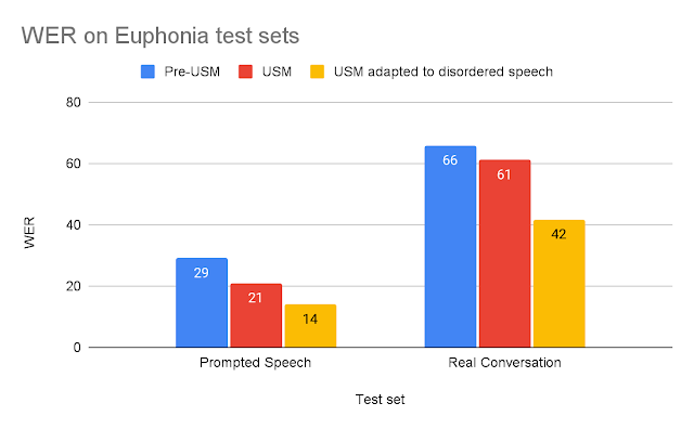
Chirp is Google’s family of state-of-the-art Universal Speech Models trained on 12 million hours of speech to enable automatic speech recognition (ASR) for 100+ languages. The models can perform ASR on under-resourced languages, such as Amharic, Cebuano, and Assamese, in addition to widely spoken languages like English and Mandarin. Chirp is able to cover such a wide variety of languages by leveraging self-supervised learning on unlabeled multilingual dataset with fine-tuning on a smaller set of labeled data. Chirp is now available in the Google Cloud Speech-to-Text API, allowing users to perform inference on the model through a simple interface. You can get started with Chirp here.

MusicLM

At I/O, we launched MusicLM, a text-to-music model that generates 20 seconds of music from a text prompt. You can try it yourself on AI Test Kitchen, or see it featured during the I/O preshow, where electronic musician and composer Dan Deacon used MusicLM in his performance.

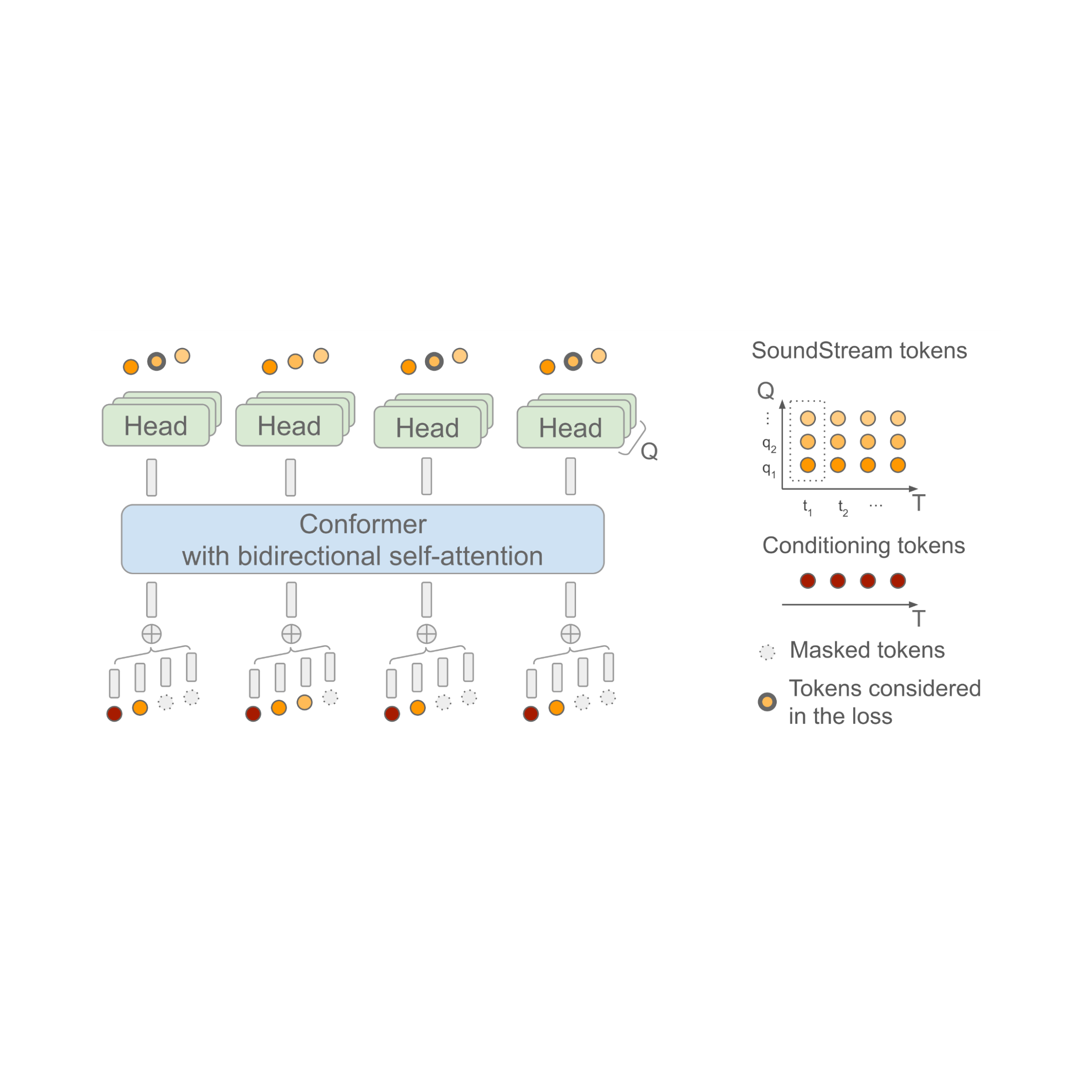
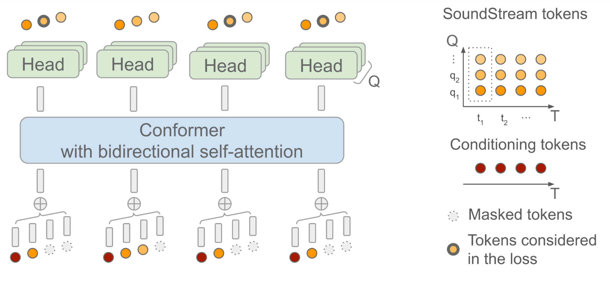
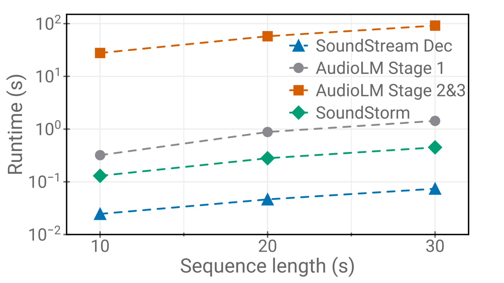
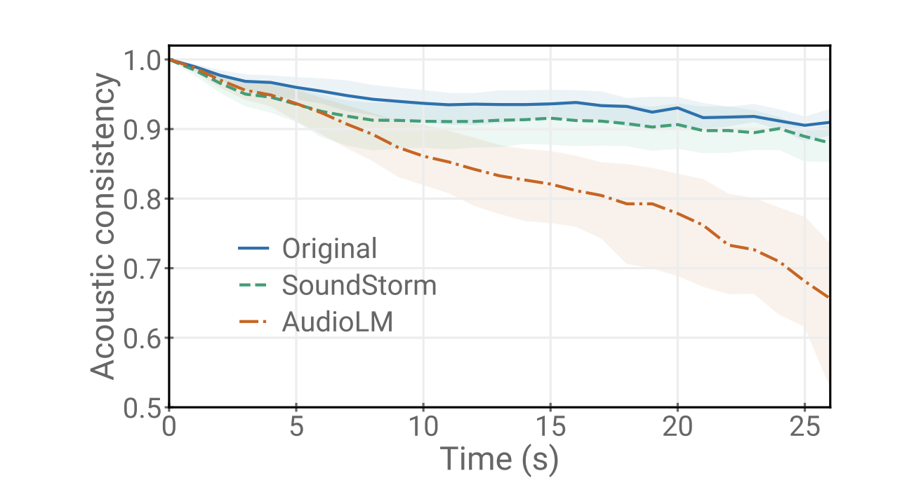
MusicLM, which consists of models powered by AudioLM and MuLAN, can make music (from text, humming, images or video) and musical accompaniments to singing. AudioLM generates high quality audio with long-term consistency. It maps audio to a sequence of discrete tokens and casts audio generation as a language modeling task. To synthesize longer outputs efficiently, it used a novel approach we’ve developed called SoundStorm.

Universal Translator dubbing

Our dubbing efforts leverage dozens of ML technologies to translate the full expressive range of video content, making videos accessible to audiences across the world. These technologies have been used to dub videos across a variety of products and content types, including educational content, advertising campaigns, and creator content, with more to come. We use deep learning technology to achieve voice preservation and lip matching and enable high-quality video translation. We’ve built this product to include human review for quality, safety checks to help prevent misuse, and we make it accessible only to authorized partners.

AI for global societal good

We are applying our AI technologies to solve some of the biggest global challenges, like mitigating climate change, adapting to a warming planet and improving human health and wellbeing. For example:

  • Traffic engineers use our Green Light recommendations to reduce stop-and-go traffic at intersections and improve the flow of traffic in cities from Bangalore to Rio de Janeiro and Hamburg. Green Light models each intersection, analyzing traffic patterns to develop recommendations that make traffic lights more efficient — for example, by better synchronizing timing between adjacent lights, or adjusting the “green time” for a given street and direction.
  • We’ve also expanded global coverage on the Flood Hub to 80 countries, as part of our efforts to predict riverine floods and alert people who are about to be impacted before disaster strikes. Our flood forecasting efforts rely on hydrological models informed by satellite observations, weather forecasts and in-situ measurements.

Technologies for inclusive and fair ML applications

With our continued investment in AI technologies, we are emphasizing responsible AI development with the goal of making our models and tools useful and impactful while also ensuring fairness, safety and alignment with our AI Principles. Some of these efforts were highlighted at I/O, including:

  • The release of the Monk Skin Tone Examples (MST-E) Dataset to help practitioners gain a deeper understanding of the MST scale and train human annotators for more consistent, inclusive, and meaningful skin tone annotations. You can read more about this and other developments on our website. This is an advancement on the open source release of the Monk Skin Tone (MST) Scale we launched last year to enable developers to build products that are more inclusive and that better represent their diverse users.
  • A new Kaggle competition (open until August 10th) in which the ML community is tasked with creating a model that can quickly and accurately identify American Sign Language (ASL) fingerspelling — where each letter of a word is spelled out in ASL rapidly using a single hand, rather than using the specific signs for entire words — and translate it into written text. Learn more about the fingerspelling Kaggle competition, which features a song from Sean Forbes, a deaf musician and rapper. We also showcased at I/O the winning algorithm from the prior year’s competition powers PopSign, an ASL learning app for parents of deaf or hard of hearing children created by Georgia Tech and Rochester Institute of Technology (RIT).

Building the future of AI together

It’s inspiring to be part of a community of so many talented individuals who are leading the way in developing state-of-the-art technologies, responsible AI approaches and exciting user experiences. We are in the midst of a period of incredible and transformative change for AI. Stay tuned for more updates about the ways in which the Google Research community is boldly exploring the frontiers of these technologies and using them responsibly to benefit people’s lives around the world. We hope you’re as excited as we are about the future of AI technologies and we invite you to engage with our teams through the references, sites and tools that we’ve highlighted here.

Categories
Offsites

Resolving code review comments with ML

Code-change reviews are a critical part of the software development process at scale, taking a significant amount of the code authors’ and the code reviewers’ time. As part of this process, the reviewer inspects the proposed code and asks the author for code changes through comments written in natural language. At Google, we see millions of reviewer comments per year, and authors require an average of ~60 minutes active shepherding time between sending changes for review and finally submitting the change. In our measurements, the required active work time that the code author must do to address reviewer comments grows almost linearly with the number of comments. However, with machine learning (ML), we have an opportunity to automate and streamline the code review process, e.g., by proposing code changes based on a comment’s text.

Today, we describe applying recent advances of large sequence models in a real-world setting to automatically resolve code review comments in the day-to-day development workflow at Google (publication forthcoming). As of today, code-change authors at Google address a substantial amount of reviewer comments by applying an ML-suggested edit. We expect that to reduce time spent on code reviews by hundreds of thousands of hours annually at Google scale. Unsolicited, very positive feedback highlights that the impact of ML-suggested code edits increases Googlers’ productivity and allows them to focus on more creative and complex tasks.

Predicting the code edit

We started by training a model that predicts code edits needed to address reviewer comments. The model is pre-trained on various coding tasks and related developer activities (e.g., renaming a variable, repairing a broken build, editing a file). It’s then fine-tuned for this specific task with reviewed code changes, the reviewer comments, and the edits the author performed to address those comments.

An example of an ML-suggested edit of refactorings that are spread within the code.

Google uses a monorepo, a single repository for all of its software artifacts, which allows our training dataset to include all unrestricted code used to build Google’s most recent software, as well as previous versions.

To improve the model quality, we iterated on the training dataset. For example, we compared the model performance for datasets with a single reviewer comment per file to datasets with multiple comments per file, and experimented with classifiers to clean up the training data based on a small, curated dataset to choose the model with the best offline precision and recall metrics.

Serving infrastructure and user experience

We designed and implemented the feature on top of the trained model, focusing on the overall user experience and developer efficiency. As part of this, we explored different user experience (UX) alternatives through a series of user studies. We then refined the feature based on insights from an internal beta (i.e., a test of the feature in development) including user feedback (e.g., a “Was this helpful?” button next to the suggested edit).

The final model was calibrated for a target precision of 50%. That is, we tuned the model and the suggestions filtering, so that 50% of suggested edits on our evaluation dataset are correct. In general, increasing the target precision reduces the number of shown suggested edits, and decreasing the target precision leads to more incorrect suggested edits. Incorrect suggested edits take the developers time and reduce the developers’ trust in the feature. We found that a target precision of 50% provides a good balance.

At a high level, for every new reviewer comment, we generate the model input in the same format that is used for training, query the model, and generate the suggested code edit. If the model is confident in the prediction and a few additional heuristics are satisfied, we send the suggested edit to downstream systems. The downstream systems, i.e., the code review frontend and the integrated development environment (IDE), expose the suggested edits to the user and log user interactions, such as preview and apply events. A dedicated pipeline collects these logs and generates aggregate insights, e.g., the overall acceptance rates as reported in this blog post.

Architecture of the ML-suggested edits infrastructure. We process code and infrastructure from multiple services, get the model predictions and surface the predictions in the code review tool and IDE.

The developer interacts with the ML-suggested edits in the code review tool and the IDE. Based on insights from the user studies, the integration into the code review tool is most suitable for a streamlined review experience. The IDE integration provides additional functionality and supports 3-way merging of the ML-suggested edits (left in the figure below) in case of conflicting local changes on top of the reviewed code state (right) into the merge result (center).

3-way-merge UX in IDE.

Results

Offline evaluations indicate that the model addresses 52% of comments with a target precision of 50%. The online metrics of the beta and the full internal launch confirm these offline metrics, i.e., we see model suggestions above our target model confidence for around 50% of all relevant reviewer comments. 40% to 50% of all previewed suggested edits are applied by code authors.

We used the “not helpful” feedback during the beta to identify recurring failure patterns of the model. We implemented serving-time heuristics to filter these and, thus, reduce the number of shown incorrect predictions. With these changes, we traded quantity for quality and observed an increased real-world acceptance rate.

Code review tool UX. The suggestion is shown as part of the comment and can be previewed, applied and rated as helpful or not helpful.

Our beta launch showed a discoverability challenge: code authors only previewed ~20% of all generated suggested edits. We modified the UX and introduced a prominent “Show ML-edit” button (see the figure above) next to the reviewer comment, leading to an overall preview rate of ~40% at launch. We additionally found that suggested edits in the code review tool are often not applicable due to conflicting changes that the author did during the review process. We addressed this with a button in the code review tool that opens the IDE in a merge view for the suggested edit. We now observe that more than 70% of these are applied in the code review tool and fewer than 30% are applied in the IDE. All these changes allowed us to increase the overall fraction of reviewer comments that are addressed with an ML-suggested edit by a factor of 2 from beta to the full internal launch. At Google scale, these results help automate the resolution of hundreds of thousands of comments each year.

Suggestions filtering funnel.

We see ML-suggested edits addressing a wide range of reviewer comments in production. This includes simple localized refactorings and refactorings that are spread within the code, as shown in the examples throughout the blog post above. The feature addresses longer and less formally-worded comments that require code generation, refactorings and imports.

Example of a suggestion for a longer and less formally worded comment that requires code generation, refactorings and imports.

The model can also respond to complex comments and produce extensive code edits (shown below). The generated test case follows the existing unit test pattern, while changing the details as described in the comment. Additionally, the edit suggests a comprehensive name for the test reflecting the test semantics.

Example of the model’s ability to respond to complex comments and produce extensive code edits.

Conclusion and future work

In this post, we introduced an ML-assistance feature to reduce the time spent on code review related changes. At the moment, a substantial amount of all actionable code review comments on supported languages are addressed with applied ML-suggested edits at Google. A 12-week A/B experiment across all Google developers will further measure the impact of the feature on the overall developer productivity.

We are working on improvements throughout the whole stack. This includes increasing the quality and recall of the model and building a more streamlined experience for the developer with improved discoverability throughout the review process. As part of this, we are investigating the option of showing suggested edits to the reviewer while they draft comments and expanding the feature into the IDE to enable code-change authors to get suggested code edits for natural-language commands.

Acknowledgements

This is the work of many people in Google Core Systems & Experiences team, Google Research, and DeepMind. We’d like to specifically thank Peter Choy for bringing the collaboration together, and all of our team members for their key contributions and useful advice, including Marcus Revaj, Gabriela Surita, Maxim Tabachnyk, Jacob Austin, Nimesh Ghelani, Dan Zheng, Peter Josling, Mariana Stariolo, Chris Gorgolewski, Sascha Varkevisser, Katja Grünwedel, Alberto Elizondo, Tobias Welp, Paige Bailey, Pierre-Antoine Manzagol, Pascal Lamblin, Chenjie Gu, Petros Maniatis, Henryk Michalewski, Sara Wiltberger, Ambar Murillo, Satish Chandra, Madhura Dudhgaonkar, Niranjan Tulpule, Zoubin Ghahramani, Juanjo Carin, Danny Tarlow, Kevin Villela, Stoyan Nikolov, David Tattersall, Boris Bokowski, Kathy Nix, Mehdi Ghissassi, Luis C. Cobo, Yujia Li, David Choi, Kristóf Molnár, Vahid Meimand, Amit Patel, Brett Wiltshire, Laurent Le Brun, Mingpan Guo, Hermann Loose, Jonas Mattes, Savinee Dancs. Thanks to John Guilyard for creating the graphics in this post.

Categories
Offsites

Making ML models differentially private: Best practices and open challenges

Large machine learning (ML) models are ubiquitous in modern applications: from spam filters to recommender systems and virtual assistants. These models achieve remarkable performance partially due to the abundance of available training data. However, these data can sometimes contain private information, including personal identifiable information, copyright material, etc. Therefore, protecting the privacy of the training data is critical to practical, applied ML.

Differential Privacy (DP) is one of the most widely accepted technologies that allows reasoning about data anonymization in a formal way. In the context of an ML model, DP can guarantee that each individual user’s contribution will not result in a significantly different model. A model’s privacy guarantees are characterized by a tuple (ε, δ), where smaller values of both represent stronger DP guarantees and better privacy.

While there are successful examples of protecting training data using DP, obtaining good utility with differentially private ML (DP-ML) techniques can be challenging. First, there are inherent privacy/computation tradeoffs that may limit a model’s utility. Further, DP-ML models often require architectural and hyperparameter tuning, and guidelines on how to do this effectively are limited or difficult to find. Finally, non-rigorous privacy reporting makes it challenging to compare and choose the best DP methods.

In “How to DP-fy ML: A Practical Guide to Machine Learning with Differential Privacy”, to appear in the Journal of Artificial Intelligence Research, we discuss the current state of DP-ML research. We provide an overview of common techniques for obtaining DP-ML models and discuss research, engineering challenges, mitigation techniques and current open questions. We will present tutorials based on this work at ICML 2023 and KDD 2023.

DP-ML methods

DP can be introduced during the ML model development process in three places: (1) at the input data level, (2) during training, or (3) at inference. Each option provides privacy protections at different stages of the ML development process, with the weakest being when DP is introduced at the prediction level and the strongest being when introduced at the input level. Making the input data differentially private means that any model that is trained on this data will also have DP guarantees. When introducing DP during the training, only that particular model has DP guarantees. DP at the prediction level means that only the model’s predictions are protected, but the model itself is not differentially private.

The task of introducing DP gets progressively easier from the left to right.

DP is commonly introduced during training (DP-training). Gradient noise injection methods, like DP-SGD or DP-FTRL, and their extensions are currently the most practical methods for achieving DP guarantees in complex models like large deep neural networks.

DP-SGD builds off of the stochastic gradient descent (SGD) optimizer with two modifications: (1) per-example gradients are clipped to a certain norm to limit sensitivity (the influence of an individual example on the overall model), which is a slow and computationally intensive process, and (2) a noisy gradient update is formed by taking aggregated gradients and adding noise that is proportional to the sensitivity and the strength of privacy guarantees.

DP-SGD is a modification of SGD that involves a) clipping per-example gradients to limit the sensitivity and b) adding the noise, calibrated to the sensitivity and privacy guarantees, to the aggregated gradients, before the gradient update step.

Existing DP-training challenges

Gradient noise injection methods usually exhibit: (1) loss of utility, (2) slower training, and (3) an increased memory footprint.

Loss of utility:

The best method for reducing utility drop is to use more computation. Using larger batch sizes and/or more iterations is one of the most prominent and practical ways of improving a model’s performance. Hyperparameter tuning is also extremely important but often overlooked. The utility of DP-trained models is sensitive to the total amount of noise added, which depends on hyperparameters, like the clipping norm and batch size. Additionally, other hyperparameters like the learning rate should be re-tuned to account for noisy gradient updates.

Another option is to obtain more data or use public data of similar distribution. This can be done by leveraging publicly available checkpoints, like ResNet or T5, and fine-tuning them using private data.

Slower training:

Most gradient noise injection methods limit sensitivity via clipping per-example gradients, considerably slowing down backpropagation. This can be addressed by choosing an efficient DP framework that efficiently implements per-example clipping.

Increased memory footprint:

DP-training requires significant memory for computing and storing per-example gradients. Additionally, it requires significantly larger batches to obtain better utility. Increasing the computation resources (e.g., the number and size of accelerators) is the simplest solution for extra memory requirements. Alternatively, several works advocate for gradient accumulation where smaller batches are combined to simulate a larger batch before the gradient update is applied. Further, some algorithms (e.g., ghost clipping, which is based on this paper) avoid per-example gradient clipping altogether.

Best practices

The following best practices can attain rigorous DP guarantees with the best model utility possible.

Choosing the right privacy unit:

First, we should be clear about a model’s privacy guarantees. This is encoded by selecting the “privacy unit,” which represents the neighboring dataset concept (i.e., datasets where only one row is different). Example-level protection is a common choice in the research literature, but may not be ideal, however, for user-generated data if individual users contributed multiple records to the training dataset. For such a case, user-level protection might be more appropriate. For text and sequence data, the choice of the unit is harder since in most applications individual training examples are not aligned to the semantic meaning embedded in the text.

Choosing privacy guarantees:

We outline three broad tiers of privacy guarantees and encourage practitioners to choose the lowest possible tier below:

  • Tier 1 — Strong privacy guarantees: Choosing ε ≤ 1 provides a strong privacy guarantee, but frequently results in a significant utility drop for large models and thus may only be feasible for smaller models.
  • Tier 2 — Reasonable privacy guarantees: We advocate for the currently undocumented, but still widely used, goal for DP-ML models to achieve an ε ≤ 10.
  • Tier 3 — Weak privacy guarantees: Any finite ε is an improvement over a model with no formal privacy guarantee. However, for ε > 10, the DP guarantee alone cannot be taken as sufficient evidence of data anonymization, and additional measures (e.g., empirical privacy auditing) may be necessary to ensure the model protects user data.

Hyperparameter tuning:

Choosing hyperparameters requires optimizing over three inter-dependent objectives: 1) model utility, 2) privacy cost ε, and 3) computation cost. Common strategies take two of the three as constraints, and focus on optimizing the third. We provide methods that will maximize the utility with a limited number of trials, e.g., tuning with privacy and computation constraints.

Reporting privacy guarantees:

A lot of works on DP for ML report only ε and possibly δ values for their training procedure. However, we believe that practitioners should provide a comprehensive overview of model guarantees that includes:

  1. DP setting: Are the results assuming central DP with a trusted service provider, local DP, or some other setting?
  2. Instantiating the DP definition:
    1. Data accesses covered: Whether the DP guarantee applies (only) to a single training run or also covers hyperparameter tuning etc.
    2. Final mechanism’s output: What is covered by the privacy guarantees and can be released publicly (e.g., model checkpoints, the full sequence of privatized gradients, etc.)
    3. Unit of privacy: The selected “privacy unit” (example-level, user-level, etc.)
    4. Adjacency definition for DP “neighboring” datasets: A description of how neighboring datasets differ (e.g., add-or-remove, replace-one, zero-out-one).
  3. Privacy accounting details: Providing accounting details, e.g., composition and amplification, are important for proper comparison between methods and should include:
    1. Type of accounting used, e.g., Rényi DP-based accounting, PLD accounting, etc.
    2. Accounting assumptions and whether they hold (e.g., Poisson sampling was assumed for privacy amplification but data shuffling was used in training).
    3. Formal DP statement for the model and tuning process (e.g., the specific ε, δ-DP or ρ-zCDP values).
  4. Transparency and verifiability: When possible, complete open-source code using standard DP libraries for the key mechanism implementation and accounting components.

Paying attention to all the components used:

Usually, DP-training is a straightforward application of DP-SGD or other algorithms. However, some components or losses that are often used in ML models (e.g., contrastive losses, graph neural network layers) should be examined to ensure privacy guarantees are not violated.

Open questions

While DP-ML is an active research area, we highlight the broad areas where there is room for improvement.

Developing better accounting methods:

Our current understanding of DP-training ε, δ guarantees relies on a number of techniques, like Rényi DP composition and privacy amplification. We believe that better accounting methods for existing algorithms will demonstrate that DP guarantees for ML models are actually better than expected.

Developing better algorithms:

The computational burden of using gradient noise injection for DP-training comes from the need to use larger batches and limit per-example sensitivity. Developing methods that can use smaller batches or identifying other ways (apart from per-example clipping) to limit the sensitivity would be a breakthrough for DP-ML.

Better optimization techniques:

Directly applying the same DP-SGD recipe is believed to be suboptimal for adaptive optimizers because the noise added to privatize the gradient may accumulate in learning rate computation. Designing theoretically grounded DP adaptive optimizers remains an active research topic. Another potential direction is to better understand the surface of DP loss, since for standard (non-DP) ML models flatter regions have been shown to generalize better.

Identifying architectures that are more robust to noise:

There’s an opportunity to better understand whether we need to adjust the architecture of an existing model when introducing DP.

Conclusion

Our survey paper summarizes the current research related to making ML models DP, and provides practical tips on how to achieve the best privacy-utility trade offs. Our hope is that this work will serve as a reference point for the practitioners who want to effectively apply DP to complex ML models.

Acknowledgements

We thank Hussein Hazimeh, Zheng Xu , Carson Denison , H. Brendan McMahan, Sergei Vassilvitskii, Steve Chien and Abhradeep Thakurta, Badih Ghazi, Chiyuan Zhang for the help preparing this blog post, paper and tutorials content. Thanks to John Guilyard for creating the graphics in this post, and Ravi Kumar for comments.

Categories
Offsites

Sparse video tubes for joint video and image vision transformers

Video understanding is a challenging problem that requires reasoning about both spatial information (e.g., for objects in a scene, including their locations and relations) and temporal information for activities or events shown in a video. There are many video understanding applications and tasks, such as understanding the semantic content of web videos and robot perception. However, current works, such as ViViT and TimeSFormer, densely process the video and require significant compute, especially as model size plus video length and resolution increase.

In “Rethinking Video ViTs: Sparse Video Tubes for Joint Image and Video Learning”, to be presented at CVPR 2023, we introduce a simple technique that turns a Vision Transformer (ViT) model image encoder into an efficient video backbone using sparse video tubes (learnable visual representations of samples from the video) to reduce the model’s compute needs. This approach can seamlessly process both images and videos, which allows it to leverage both image and video data sources during training. This training further enables our sparse tubes ViT model to coalesce image and video backbones together to serve a dual role as either an image or video backbone (or both), depending on the input. We demonstrate that this model is scalable, can be adapted to large pre-trained ViTs without requiring full fine-tuning, and achieves state-of-the-art results across many video classification benchmarks.

Using sparse video tubes to sample a video, combined with a standard ViT encoder, leads to an efficient visual representation that can be seamlessly shared with image inputs.

Building a joint image-video backbone

Our sparse tube ViT uses a standard ViT backbone, consisting of a stack of Transformer layers, that processes video information. Previous methods, such as ViViT, densely tokenize the video and then apply factorized attention, i.e., the attention weights for each token are computed separately for the temporal and spatial dimensions. In the standard ViT architecture, self-attention is computed over the whole token sequence. When using videos as input, token sequences become quite long, which can make this computation slow. Instead, in the method we propose, the video is sparsely sampled using video tubes, which are 3D learnable visual representations of various shapes and sizes (described in more detail below) from the video. These tubes are used to sparsely sample the video using a large temporal stride, i.e., when a tube kernel is only applied to a few locations in the video, rather than every pixel.

By sparsely sampling the video tubes, we can use the same global self-attention module, rather than factorized attention like ViViT. We experimentally show that the addition of factorized attention layers can harm the performance due to the uninitialized weights. This single stack of transformer layers in the ViT backbone also enables better sharing of the weights and improves performance. Sparse video tube sampling is done by using a large spatial and temporal stride that selects tokens on a fixed grid. The large stride reduces the number of tokens in the full network, while still capturing both spatial and temporal information and enabling the efficient processing of all tokens.

Sparse video tubes

Video tubes are 3D grid-based cuboids that can have different shapes or categories and capture different information with strides and starting locations that can overlap. In the model, we use three distinct tube shapes that capture: (1) only spatial information (resulting in a set of 2D image patches), (2) long temporal information (over a small spatial area), and (3) both spatial and temporal information equally. Tubes that capture only spatial information can be applied to both image and video inputs. Tubes that capture long temporal information or both temporal and spatial information equally are only applied to video inputs. Depending on the input video size, the three tube shapes are applied to the model multiple times to generate tokens.

A fixed position embedding, which captures the global location of each tube (including any strides, offsets, etc.) relative to all the other tubes, is applied to the video tubes. Different from the previous learned position embeddings, this fixed one better enables sparse, overlapping sampling. Capturing the global location of the tube helps the model know where each came from, which is especially helpful when tubes overlap or are sampled from distant video locations. Next, the tube features are concatenated together to form a set of N tokens. These tokens are processed by a standard ViT encoder. Finally, we apply an attention pooling to compress all the tokens into a single representation and input to a fully connected (FC) layer to make the classification (e.g., playing soccer, swimming, etc.).

Our video ViT model works by sampling sparse video tubes from the video (shown at the bottom) to enable either or both image or video inputs to be seamlessly processed. These tubes have different shapes and capture different video features. Tube 1 (yellow) only captures spatial information, resulting in a set of 2D patches that can be applied to image inputs. Tube 2 (red) captures temporal information and some spatial information and tube 3 (green) equally captures both temporal and spatial information (i.e., the spatial size of the tube x and y are the same as the number of frames t). Tubes 2 and 3 can only be applied to video inputs. The position embedding is added to all the tube features.

Scaling video ViTs

The process of building video backbones is computationally intensive, but our sparse tube ViT model enables computationally efficient scaling of video models, leveraging previously trained image backbones. Since image backbones can be adapted to a video backbone, large image backbones can be turned into large video backbones. More specifically, one can transfer the learned video feature representations from a small tube ViT to a large pre-trained image ViT and train the resulting model with video data for only a few steps, as opposed to a full training from scratch.

Our approach enables scaling a sparse tube ViT in a more efficient way. Specifically, the video features from a small video ViT (top network) can be transferred to a large, pre-trained image ViT (bottom network), and further fine-tuned. This requires fewer training steps to achieve strong performance with the large model. This is beneficial as large video models might be prohibitively expensive to train from scratch.

Results

We evaluate our sparse tube ViT approach using Kinetics-400 (shown below), Kinetics-600 and Kinetics-700 datasets and compare its performance to a long list of prior methods. We find that our approach outperforms all prior methods. Importantly, it outperforms all state-of-the-art methods trained jointly on image+video datasets.

Performance compared to several prior works on the popular Kinetics-400 video dataset. Our sparse tube ViT outperforms state-of-the-art methods.

Furthermore, we test our sparse tube ViT model on the Something-Something V2 dataset, which is commonly used to evaluate more dynamic activities, and also report that it outperforms all prior state-of-the-art approaches.

Performance on the Something-Something V2 video dataset.

Visualizing some learned kernels

It is interesting to understand what kind of rudimentary features are being learned by the proposed model. We visualize them below, showing both the 2D patches, which are shared for both images and videos, and video tubes. These visualizations show the 2D or 3D information being captured by the projection layer. For example, in the 2D patches, various common features, like edges and colors, are detected, while the 3D tubes capture basic shapes and how they may change over time.

Visualizations of patches and tubes learned the sparse tube ViT model. Top row are the 2D patches and the remaining two rows are snapshots from the learned video tubes. The tubes show each patch for the 8 or 4 frames to which they are applied.

Conclusions

We have presented a new sparse tube ViT, which can turn a ViT encoder into an efficient video model, and can seamlessly work with both image and video inputs. We also showed that large video encoders can be bootstrapped from small video encoders and image-only ViTs. Our approach outperforms prior methods across several popular video understanding benchmarks. We believe that this simple representation can facilitate much more efficient learning with input videos, seamlessly incorporate either image or video inputs and effectively eliminate the bifurcation of image and video models for future multimodal understanding.

Acknowledgements

This work is conducted by AJ Piergiovanni, Weicheng Kuo and Anelia Angelova, who are now at Google DeepMind. We thank Abhijit Ogale, Luowei Zhou, Claire Cui and our colleagues in Google Research for their helpful discussions, comments, and support.

Categories
Offsites

Foundation models for reasoning on charts

Visual language is the form of communication that relies on pictorial symbols outside of text to convey information. It is ubiquitous in our digital life in the form of iconography, infographics, tables, plots, and charts, extending to the real world in street signs, comic books, food labels, etc. For that reason, having computers better understand this type of media can help with scientific communication and discovery, accessibility, and data transparency.

While computer vision models have made tremendous progress using learning-based solutions since the advent of ImageNet, the focus has been on natural images, where all sorts of tasks, such as classification, visual question answering (VQA), captioning, detection and segmentation, have been defined, studied and in some cases advanced to reach human performance. However, visual language has not garnered a similar level of attention, possibly because of the lack of large-scale training sets in this space. But over the last few years, new academic datasets have been created with the goal of evaluating question answering systems on visual language images, like PlotQA, InfographicsVQA, and ChartQA.

Example from ChartQA. Answering the question requires reading the information and computing the sum and the difference.

Existing models built for these tasks relied on integrating optical character recognition (OCR) information and their coordinates into larger pipelines but the process is error prone, slow, and generalizes poorly. The prevalence of these methods was because existing end-to-end computer vision models based on convolutional neural networks (CNNs) or transformers pre-trained on natural images could not be easily adapted to visual language. But existing models are ill-prepared for the challenges in answering questions on charts, including reading the relative height of bars or the angle of slices in pie charts, understanding axis scales, correctly mapping pictograms with their legend values with colors, sizes and textures, and finally performing numerical operations with the extracted numbers.

In light of these challenges, we propose “MatCha: Enhancing Visual Language Pretraining with Math Reasoning and Chart Derendering”. MatCha, which stands for math and charts, is a pixels-to-text foundation model (a pre-trained model with built-in inductive biases that can be fine-tuned for multiple applications) trained on two complementary tasks: (a) chart de-rendering and (b) math reasoning. In chart de-rendering, given a plot or chart, the image-to-text model is required to generate its underlying data table or the code used to render it. For math reasoning pre-training, we pick textual numerical reasoning datasets and render the input into images, which the image-to-text model needs to decode for answers. We also propose “DePlot: One-shot visual language reasoning by plot-to-table translation”, a model built on top of MatCha for one-shot reasoning on charts via translation to tables. With these methods we surpass the previous state of the art in ChartQA by more than 20% and match the best summarization systems that have 1000 times more parameters. Both papers will be presented at ACL2023.

Chart de-rendering

Plots and charts are usually generated by an underlying data table and a piece of code. The code defines the overall layout of the figure (e.g., type, direction, color/shape scheme) and the underlying data table establishes the actual numbers and their groupings. Both the data and code are sent to a compiler/rendering engine to create the final image. To understand a chart, one needs to discover the visual patterns in the image and effectively parse and group them to extract the key information. Reversing the plot rendering process demands all such capabilities and can thus serve as an ideal pre-training task.

A chart created from a table in the Airbus A380 Wikipedia page using random plotting options. The pre-training task for MatCha consists of recovering the source table or the source code from the image.

In practice, it is challenging to simultaneously obtain charts, their underlying data tables, and their rendering code. To collect sufficient pre-training data, we independently accumulate [chart, code] and [chart, table] pairs. For [chart, code], we crawl all GitHub IPython notebooks with appropriate licenses and extract blocks with figures. A figure and the code block right before it are saved as a [chart, code] pair. For [chart, table] pairs, we explored two sources. For the first source, synthetic data, we manually write code to convert web-crawled Wikipedia tables from the TaPas codebase to charts. We sampled from and combined several plotting options depending on the column types. In addition, we also add [chart, table] pairs generated in PlotQA to diversify the pre-training corpus. The second source is web-crawled [chart, table] pairs. We directly use the [chart, table] pairs crawled in the ChartQA training set, containing around 20k pairs in total from four websites: Statista, Pew, Our World in Data, and OECD.

Math reasoning

We incorporate numerical reasoning knowledge into MatCha by learning math reasoning skills from textual math datasets. We use two existing textual math reasoning datasets, MATH and DROP for pre-training. MATH is synthetically created, containing two million training examples per module (type) of questions. DROP is a reading-comprehension–style QA dataset where the input is a paragraph context and a question.

To solve questions in DROP, the model needs to read the paragraph, extract relevant numbers and perform numerical computation. We found both datasets to be complementary. MATH contains a large number of questions across different categories, which helps us identify math operations needed to explicitly inject into the model. DROP’s reading-comprehension format resembles the typical QA format wherein models simultaneously perform information extraction and reasoning. In practice, we render inputs of both datasets into images. The model is trained to decode the answer.

To improve the math reasoning skills of MatCha we incorporate examples from MATH and DROP into the pre-training objective, by rendering the input text as images.

End-to-end results

We use a Pix2Struct model backbone, which is an image-to-text transformer tailored for website understanding, and pre-train it with the two tasks described above. We demonstrate the strengths of MatCha by fine-tuning it on several visual language tasks — tasks involving charts and plots for question answering and summarization where no access to the underlying table is possible. MatCha surpasses previous models’ performance by a large margin and also outperforms the previous state of the art, which assumes access to underlying tables.

In the figure below, we first evaluate two baseline models that incorporate information from an OCR pipeline, which until recently was the standard approach for working with charts. The first is based on T5, the second on VisionTaPas. We also compare against PaLI-17B, which is a large (~1000 times larger than the other models) image plus text-to-text transformer trained on a diverse set of tasks but with limited capabilities for reading text and other forms of visual language. Finally, we report the Pix2Struct and MatCha model results.

Experimental results on two chart QA benchmarks ChartQA & PlotQA (using relaxed accuracy) and a chart summarization benchmark chart-to-text (using BLEU4). Matcha surpasses the state of the art by a large margin on QA, compared to larger models, and matches these larger models on summarization.

For QA datasets, we use the official relaxed accuracy metric that allows for small relative errors in numerical outputs. For chart-to-text summarization, we report BLEU scores. MatCha achieves noticeably improved results compared to baselines for question answering, and comparable results to PaLI in summarization, where large size and extensive long text/captioning generation pre-training are advantageous for this kind of long-form text generation.

Derendering plus large language model chains

While extremely performant for their number of parameters, particularly on extractive tasks, we observed that fine-tuned MatCha models could still struggle with end-to-end complex reasoning (e.g., mathematical operations involving large numbers or multiple steps). Thus, we also propose a two-step method to tackle this: 1) a model reads a chart, then outputs the underlying table, 2) a large language model (LLM) reads this output and then tries to answer the question solely based on the textual input.

For the first model, we fine-tuned MatCha solely on the chart-to-table task, increasing the output sequence length to guarantee it could recover all or most of the information in the chart. DePlot is the resulting model. In the second stage, any LLM (such as FlanPaLM or Codex) can be used for the task, and we can rely on the standard methods to increase performance on LLMs, for example chain-of-thought and self-consistency. We also experimented with program-of-thoughts where the model produces executable Python code to offload complex computations.

An illustration of the DePlot+LLM method. This is a real example using FlanPaLM and Codex. The blue boxes are input to the LLM and the red boxes contain the answer generated by the LLMs. We highlight some of the key reasoning steps in each answer.

As shown in the example above, the DePlot model in combination with LLMs outperforms fine-tuned models by a significant margin, especially so in the human-sourced portion of ChartQA, where the questions are more natural but demand more difficult reasoning. Furthermore, DePlot+LLM can do so without access to any training data.

We have released the new models and code at our GitHub repo, where you can try it out yourself in colab. Checkout the papers for MatCha and DePlot for more details on the experimental results. We hope that our results can benefit the research community and make the information in charts and plots more accessible to everyone.

Acknowledgements

This work was carried out by Fangyu Liu, Julian Martin Eisenschlos, Francesco Piccinno, Syrine Krichene, Chenxi Pang, Kenton Lee, Mandar Joshi, Wenhu Chen and Yasemin Altun from our Language Team as part of Fangyu’s internship project. Nigel Collier from Cambridge also was a collaborator. We would like to thank Joshua Howland, Alex Polozov, Shrestha Basu Mallick, Massimo Nicosia and William Cohen for their valuable comments and suggestions.

Categories
Offsites

Differential Privacy Accounting by Connecting the Dots

Differential privacy (DP) is an approach that enables data analytics and machine learning (ML) with a mathematical guarantee on the privacy of user data. DP quantifies the “privacy cost” of an algorithm, i.e., the level of guarantee that the algorithm’s output distribution for a given dataset will not change significantly if a single user’s data is added to or removed from it. The algorithm is characterized by two parameters, ε and δ, where smaller values of both indicate “more private”. There is a natural tension between the privacy budget (ε, δ) and the utility of the algorithm: a smaller privacy budget requires the output to be more “noisy”, often leading to less utility. Thus, a fundamental goal of DP is to attain as much utility as possible for a desired privacy budget.

A key property of DP that often plays a central role in understanding privacy costs is that of composition, which reflects the net privacy cost of a combination of DP algorithms, viewed together as a single algorithm. A notable example is the differentially-private stochastic gradient descent (DP-SGD) algorithm. This algorithm trains ML models over multiple iterations — each of which is differentially private — and therefore requires an application of the composition property of DP. A basic composition theorem in DP says that the privacy cost of a collection of algorithms is, at most, the sum of the privacy cost of each. However, in many cases, this can be a gross overestimate, and several improved composition theorems provide better estimates of the privacy cost of composition.

In 2019, we released an open-source library (on GitHub) to enable developers to use analytic techniques based on DP. Today, we announce the addition to this library of Connect-the-Dots, a new privacy accounting algorithm based on a novel approach for discretizing privacy loss distributions that is a useful tool for understanding the privacy cost of composition. This algorithm is based on the paper “Connect the Dots: Tighter Discrete Approximations of Privacy Loss Distributions”, presented at PETS 2022. The main novelty of this accounting algorithm is that it uses an indirect approach to construct more accurate discretizations of privacy loss distributions. We find that Connect-the-Dots provides significant gains over other privacy accounting methods in literature in terms of accuracy and running time. This algorithm was also recently applied for the privacy accounting of DP-SGD in training Ads prediction models.

Differential Privacy and Privacy Loss Distributions

A randomized algorithm is said to satisfy DP guarantees if its output “does not depend significantly” on any one entry in its training dataset, quantified mathematically with parameters (ε, δ). For example, consider the motivating example of DP-SGD. When trained with (non-private) SGD, a neural network could, in principle, be encoding the entire training dataset within its weights, thereby allowing one to reconstruct some training examples from a trained model. On the other hand, when trained with DP-SGD, we have a formal guarantee that if one were able to reconstruct a training example with non-trivial probability then one would also be able to reconstruct the same example even if it was not included in the training dataset.

The hockey stick divergence, parameterized by ε, is a measure of distance between two probability distributions, as illustrated in the figure below. The privacy cost of most DP algorithms is dictated by the hockey stick divergence between two associated probability distributions P and Q. The algorithm satisfies DP with parameters (ε, δ), if the value of the hockey stick divergence for ε between P and Q is at most δ. The hockey stick divergence between (P, Q), denoted δP||Q(ε) is in turn completely characterized by it associated privacy loss distribution, denoted by PLDP||Q.

Illustration of hockey stick divergence δP||Q(ε) between distributions P and Q (left), which corresponds to the probability mass of P that is above eεQ, where eεQ is an eε scaling of the probability mass of Q (right).

The main advantage of dealing with PLDs is that compositions of algorithms correspond to the convolution of the corresponding PLDs. Exploiting this fact, prior work has designed efficient algorithms to compute the PLD corresponding to the composition of individual algorithms by simply performing convolution of the individual PLDs using the fast Fourier transform algorithm.

However, one challenge when dealing with many PLDs is that they often are continuous distributions, which make the convolution operations intractable in practice. Thus, researchers often apply various discretization approaches to approximate the PLDs using equally spaced points. For example, the basic version of the Privacy Buckets algorithm assigns the probability mass of the interval between two discretization points entirely to the higher end of the interval.

Illustration of discretization by rounding up probability masses. Here a continuous PLD (in blue) is discretized to a discrete PLD (in red), by rounding up the probability mass between consecutive points.

Connect-the-Dots : A New Algorithm

Our new Connect-the-Dots algorithm provides a better way to discretize PLDs towards the goal of estimating hockey stick divergences. This approach works indirectly by first discretizing the hockey stick divergence function and then mapping it back to a discrete PLD supported on equally spaced points.

Illustration of high-level steps in the Connect-the-Dots algorithm.

This approach relies on the notion of a “dominating PLD”, namely, PLDP’||Q’ dominates over PLDP||Q if the hockey stick divergence of the former is greater or equal to the hockey stick divergence of the latter for all values of ε. The key property of dominating PLDs is that they remain dominating after compositions. Thus for purposes of privacy accounting, it suffices to work with a dominating PLD, which gives us an upper bound on the exact privacy cost.

Our main insight behind the Connect-the-Dots algorithm is a characterization of discrete PLD, namely that a PLD is supported on a given finite set of ε values if and only if the corresponding hockey stick divergence as a function of eε is linear between consecutive eε values. This allows us to discretize the hockey stick divergence by simply connecting the dots to get a piecewise linear function that precisely equals the hockey stick divergence function at the given eε values. See a more detailed explanation of the algorithm.

Comparison of the discretizations of hockey stick divergence by Connect-the-Dots vs Privacy Buckets.

Experimental Evaluation

The DP-SGD algorithm involves a noise multiplier parameter, which controls the magnitude of noise added in each gradient step, and a sampling probability, which controls how many examples are included in each mini-batch. We compare Connect-the-Dots against the algorithms listed below on the task of privacy accounting DP-SGD with a noise multiplier = 0.5, sampling probability = 0.2 x 10⁻⁴ and δ = 10-8.

We plot the value of the ε computed by each of the algorithms against the number of composition steps, and additionally, we plot the running time of the implementations. As shown in the plots below, privacy accounting using Renyi DP provides a loose estimate of the privacy loss. However, when comparing the approaches using PLD, we find that in this example, the implementation of Connect-the-Dots achieves a tighter estimate of the privacy loss, with a running time that is 5x faster than the Microsoft PRV Accountant and >200x faster than the previous approach of Privacy Buckets in the Google-DP library.

Left: Upper bounds on the privacy parameter ε for varying number of steps of DP-SGD, as returned by different algorithms (for fixed δ = 10-8). Right: Running time of the different algorithms.

Conclusion & Future Directions

This work proposes Connect-the-Dots, a new algorithm for computing optimal privacy parameters for compositions of differentially private algorithms. When evaluated on the DP-SGD task, we find that this algorithm gives tighter estimates on the privacy loss with a significantly faster running time.

So far, the library only supports the pessimistic estimate version of Connect-the-Dots algorithm, which provides an upper bound on the privacy loss of DP-algorithms. However, the paper also introduces a variant of the algorithm that provides an “optimistic” estimate of the PLD, which can be used to derive lower bounds on the privacy cost of DP-algorithms (provided those admit a “worst case” PLD). Currently, the library does support optimistic estimates as given by the Privacy Buckets algorithm, and we hope to incorporate the Connect-the-Dots version as well.

Acknowledgements

This work was carried out in collaboration with Vadym Doroshenko, Badih Ghazi, Ravi Kumar. We thank Galen Andrew, Stan Bashtavenko, Steve Chien, Christoph Dibak, Miguel Guevara, Peter Kairouz, Sasha Kulankhina, Stefan Mellem, Jodi Spacek, Yurii Sushko and Andreas Terzis for their help.