Posted by Jeff Dean, Senior Fellow and SVP of Google Research, on behalf of the entire Google Research community
Over the last several decades, I’ve witnessed a lot of change in the fields of machine learning (ML) and computer science. Early approaches, which often fell short, eventually gave rise to modern approaches that have been very successful. Following that long-arc pattern of progress, I think we’ll see a number of exciting advances over the next several years, advances that will ultimately benefit the lives of billions of people with greater impact than ever before. In this post, I’ll highlight five areas where ML is poised to have such impact. For each, I’ll discuss related research (mostly from 2021) and the directions and progress we’ll likely see in the next few years.
<!–
–>
Trend 1: More Capable, General-Purpose ML Models
Researchers are training larger, more capable machine learning models than ever before. For example, just in the last couple of years models in the language domain have grown from billions of parameters trained on tens of billions of tokens of data (e.g., the 11B parameter T5 model), to hundreds of billions or trillions of parameters trained on trillions of tokens of data (e.g., dense models such as OpenAI’s 175B parameter GPT-3 model and DeepMind’s 280B parameter Gopher model, and sparse models such as Google’s 600B parameter GShard model and 1.2T parameter GLaM model). These increases in dataset and model size have led to significant increases in accuracy for a wide variety of language tasks, as shown by across-the-board improvements on standard natural language processing (NLP) benchmark tasks (as predicted by work on neural scaling laws for language models and machine translation models).
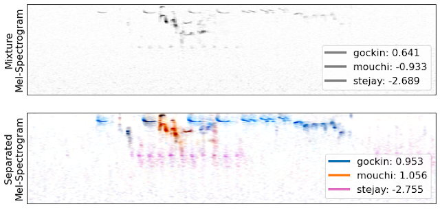
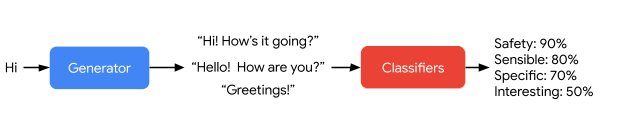
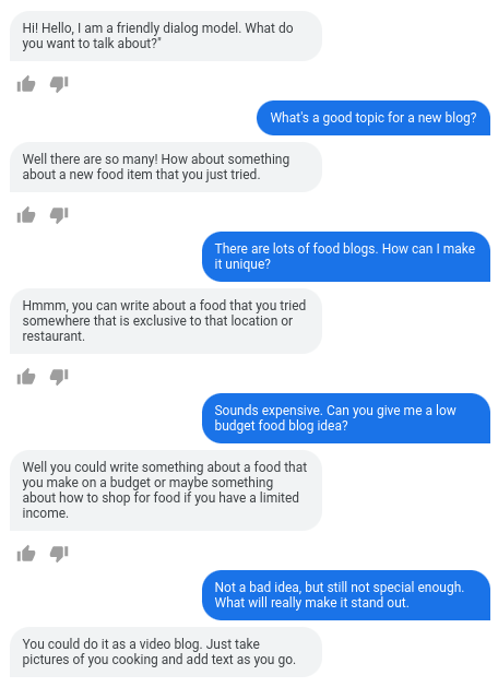
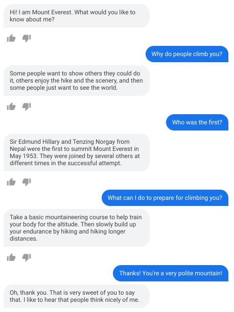
Many of these advanced models are focused on the single but important modality of written language and have shown state-of-the-art results in language understanding benchmarks and open-ended conversational abilities, even across multiple tasks in a domain. They have also shown exciting capabilities to generalize to new language tasks with relatively little training data, in some cases, with few to no training examples for a new task. A couple of examples include improved long-form question answering, zero-label learning in NLP, and our LaMDA model, which demonstrates a sophisticated ability to carry on open-ended conversations that maintain significant context across multiple turns of dialog.
 |
|
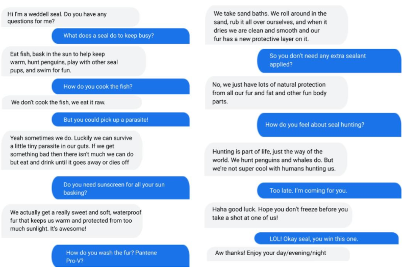 |
A dialog with LaMDA mimicking a Weddell seal with the preset grounding prompt, “Hi I’m a weddell seal. Do you have any questions for me?” The model largely holds down a dialog in character.
(Weddell Seal image cropped from Wikimedia CC licensed image.) |
Transformer models are also having a major impact in image, video, and speech models, all of which also benefit significantly from scale, as predicted by work on scaling laws for visual transformer models. Transformers for image recognition and for video classification are achieving state-of-the-art results on many benchmarks, and we’ve also demonstrated that co-training models on both image data and video data can improve performance on video tasks compared with video data alone. We’ve developed sparse, axial attention mechanisms for image and video transformers that use computation more efficiently, found better ways of tokenizing images for visual transformer models, and improved our understanding of visual transformer methods by examining how they operate compared with convolutional neural networks. Combining transformer models with convolutional operations has shown significant benefits in visual as well as speech recognition tasks.
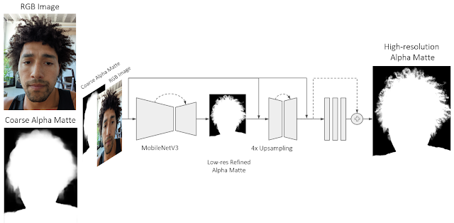
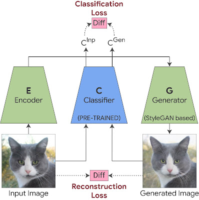
The outputs of generative models are also substantially improving. This is most apparent in generative models for images, which have made significant strides over the last few years. For example, recent models have demonstrated the ability to create realistic images given just a category (e.g., “irish setter” or “streetcar”, if you desire), can “fill in” a low-resolution image to create a natural-looking high-resolution counterpart (“computer, enhance!”), and can even create natural-looking aerial nature scenes of arbitrary length. As another example, images can be converted to a sequence of discrete tokens that can then be synthesized at high fidelity with an autoregressive generative model.
 |
| Example of a cascade diffusion models that generate novel images from a given category and then use those as the seed to create high-resolution examples: the first model generates a low resolution image, and the rest perform upsampling to the final high resolution image. |
|
| The SR3 super-resolution diffusion model takes as input a low-resolution image, and builds a corresponding high resolution image from pure noise. |
Because these are powerful capabilities that come with great responsibility, we carefully vet potential applications of these sorts of models against our AI Principles.
Beyond advanced single-modality models, we are also starting to see large-scale multi-modal models. These are some of the most advanced models to date because they can accept multiple different input modalities (e.g., language, images, speech, video) and, in some cases, produce different output modalities, for example, generating images from descriptive sentences or paragraphs, or describing the visual content of images in human languages. This is an exciting direction because like the real world, some things are easier to learn in data that is multimodal (e.g., reading about something and seeing a demonstration is more useful than just reading about it). As such, pairing images and text can help with multi-lingual retrieval tasks, and better understanding of how to pair text and image inputs can yield improved results for image captioning tasks. Similarly, jointly training on visual and textual data can also help improve accuracy and robustness on visual classification tasks, while co-training on image, video, and audio tasks improves generalization performance for all modalities. There are also tantalizing hints that natural language can be used as an input for image manipulation, telling robots how to interact with the world and controlling other software systems, portending potential changes to how user interfaces are developed. Modalities handled by these models will include speech, sounds, images, video, and languages, and may even extend to structured data, knowledge graphs, and time series data.
 |
| Example of a vision-based robotic manipulation system that is able to generalize to novel tasks. Left: The robot is performing a task described in natural language to the robot as “place grapes in ceramic bowl”, without the model being trained on that specific task. Right: As on the left, but with the novel task description of “place bottle in tray”. |
Often these models are trained using self-supervised learning approaches, where the model learns from observations of “raw” data that has not been curated or labeled, e.g., language models used in GPT-3 and GLaM, the self-supervised speech model BigSSL, the visual contrastive learning model SimCLR, and the multimodal contrastive model VATT. Self-supervised learning allows a large speech recognition model to match the previous Voice Search automatic speech recognition (ASR) benchmark accuracy while using only 3% of the annotated training data. These trends are exciting because they can substantially reduce the effort required to enable ML for a particular task, and because they make it easier (though by no means trivial) to train models on more representative data that better reflects different subpopulations, regions, languages, or other important dimensions of representation.
All of these trends are pointing in the direction of training highly capable general-purpose models that can handle multiple modalities of data and solve thousands or millions of tasks. By building in sparsity, so that the only parts of a model that are activated for a given task are those that have been optimized for it, these multimodal models can be made highly efficient. Over the next few years, we are pursuing this vision in a next-generation architecture and umbrella effort called Pathways. We expect to see substantial progress in this area, as we combine together many ideas that to date have been pursued relatively independently.
 |
| Pathways: a depiction of a single model we are working towards that can generalize across millions of tasks. |
Top
Trend 2: Continued Efficiency Improvements for ML
Improvements in efficiency — arising from advances in computer hardware design as well as ML algorithms and meta-learning research — are driving greater capabilities in ML models. Many aspects of the ML pipeline, from the hardware on which a model is trained and executed to individual components of the ML architecture, can be optimized for efficiency while maintaining or improving on state-of-the-art performance overall. Each of these different threads can improve efficiency by a significant multiplicative factor, and taken together, can reduce computational costs, including CO2 equivalent emissions (CO2e), by orders of magnitude compared to just a few years ago. This greater efficiency has enabled a number of critical advances that will continue to dramatically improve the efficiency of machine learning, enabling larger, higher quality ML models to be developed cost effectively and further democratizing access. I’m very excited about these dirctions of research!
Continued Improvements in ML Accelerator Performance
Each generation of ML accelerator improves on previous generations, enabling faster performance per chip, and often increasing the scale of the overall systems. Last year, we announced our TPUv4 systems, the fourth generation of Google’s Tensor Processing Unit, which demonstrated a 2.7x improvement over comparable TPUv3 results in the MLPerf benchmarks. Each TPUv4 chip has ~2x the peak performance per chip versus the TPUv3 chip, and the scale of each TPUv4 pod is 4096 chips (4x that of TPUv3 pods), yielding a performance of approximately 1.1 exaflops per pod (versus ~100 petaflops per TPUv3 pod). Having pods with larger numbers of chips that are connected together with high speed networks improves efficiency for larger models.
ML capabilities on mobile devices are also increasing significantly. The Pixel 6 phone features a brand new Google Tensor processor that integrates a powerful ML accelerator to better support important on-device features.
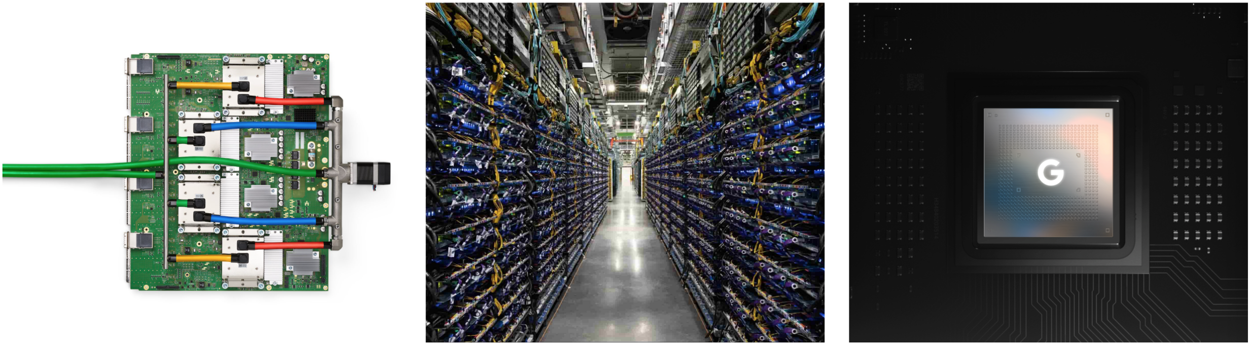 |
| Left: TPUv4 board; Center: Part of a TPUv4 pod; Right: Google Tensor chip found in Pixel 6 phones. |
Our use of ML to accelerate the design of computer chips of all kinds (more on this below) is also paying dividends, particularly to produce better ML accelerators.
Continued Improvements in ML Compilation and Optimization of ML Workloads
Even when the hardware is unchanged, improvements in compilers and other optimizations in system software for machine learning accelerators can lead to significant improvements in efficiency. For example, “A Flexible Approach to Autotuning Multi-pass Machine Learning Compilers” shows how to use machine learning to perform auto-tuning of compilation settings to get across-the-board performance improvements of 5-15% (and sometimes as much as 2.4x improvement) for a suite of ML programs on the same underlying hardware. GSPMD describes an automatic parallelization system based on the XLA compiler that is capable of scaling most deep learning network architectures beyond the memory capacity of an accelerator and has been applied to many large models, such as GShard-M4, LaMDA, BigSSL, ViT, MetNet-2, and GLaM, leading to state-of-the-art results across several domains.
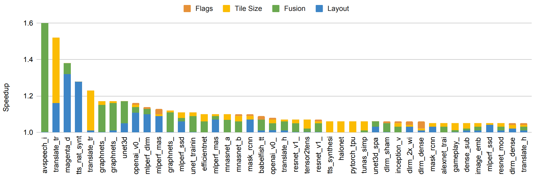 |
| End-to-end model speedups from using ML-based compiler autotuning on 150 ML models. Included are models that achieve improvements of 5% or more. Bar colors represent relative improvement from optimizing different model components. |
Human-Creativity–Driven Discovery of More Efficient Model Architectures
Continued improvements in model architectures give substantial reductions in the amount of computation needed to achieve a given level of accuracy for many problems. For example, the Transformer architecture, which we developed in 2017, was able to improve the state of the art on several NLP and translation benchmarks while simultaneously using 10x to 100x less computation to achieve these results than a variety of other prevalent methods, such as LSTMs and other recurrent architectures. Similarly, the Vision Transformer was able to show improved state-of-the-art results on a number of different image classification tasks despite using 4x to 10x less computation than convolutional neural networks.
Machine-Driven Discovery of More Efficient Model Architectures
Neural architecture search (NAS) can automatically discover new ML architectures that are more efficient for a given problem domain. A primary advantage of NAS is that it can greatly reduce the effort needed for algorithm development, because NAS requires only a one-time effort per search space and problem domain combination. In addition, while the initial effort to perform NAS can be computationally expensive, the resulting models can greatly reduce computation in downstream research and production settings, resulting in greatly reduced resource requirements overall. For example, the one-time search to discover the Evolved Transformer generated only 3.2 tons of CO2e (much less than the 284t CO2e reported elsewhere; see Appendix C and D in this joint Google/UC Berkeley preprint), but yielded a model for use by anyone in the NLP community that is 15-20% more efficient than the plain Transformer model. A more recent use of NAS discovered an even more efficient architecture called Primer (that has also been open-sourced), which reduces training costs by 4x compared to a plain Transformer model. In this way, the discovery costs of NAS searches are often recouped from the use of the more-efficient model architectures that are discovered, even if they are applied to only a handful of downstream uses (and many NAS results are reused thousands of times).
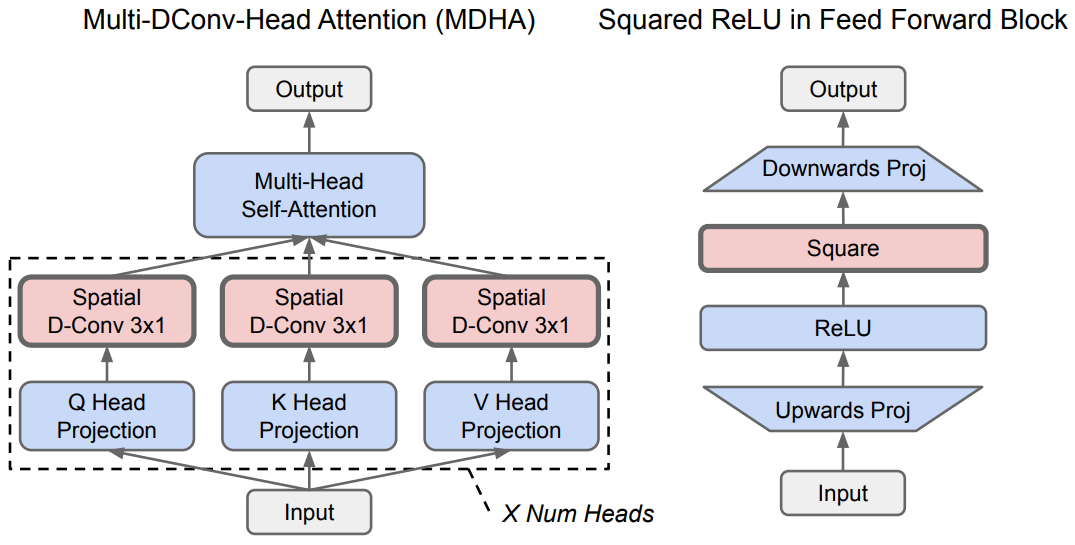 |
| The Primer architecture discovered by NAS is 4x as efficient compared with a plain Transformer model. This image shows (in red) the two main modifications that give Primer most of its gains: depthwise convolution added to attention multi-head projections and squared ReLU activations (blue indicates portions of the original Transformer). |
NAS has also been used to discover more efficient models in the vision domain. The EfficientNetV2 model architecture is the result of a neural architecture search that jointly optimizes for model accuracy, model size, and training speed. On the ImageNet benchmark, EfficientNetV2 improves training speed by 5–11x while substantially reducing model size over previous state-of-the-art models. The CoAtNet model architecture was created with an architecture search that uses ideas from the Vision Transformer and convolutional networks to create a hybrid model architecture that trains 4x faster than the Vision Transformer and achieves a new ImageNet state of the art.
The broad use of search to help improve ML model architectures and algorithms, including the use of reinforcement learning and evolutionary techniques, has inspired other researchers to apply this approach to different domains. To aid others in creating their own model searches, we have open-sourced Model Search, a platform that enables others to explore model search for their domains of interest. In addition to model architectures, automated search can also be used to find new, more efficient reinforcement learning algorithms, building on the earlier AutoML-Zero work that demonstrated this approach for automating supervised learning algorithm discovery.
Use of Sparsity
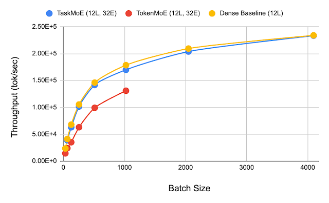
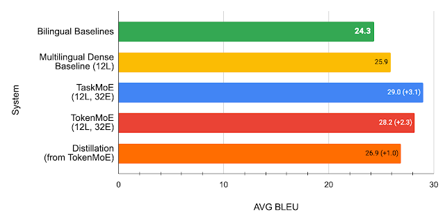
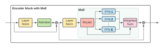
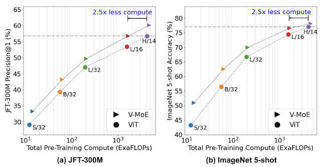
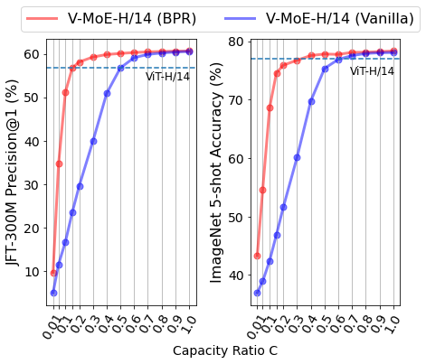
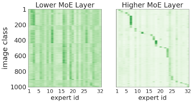
Sparsity, where a model has a very large capacity, but only some parts of the model are activated for a given task, example or token, is another important algorithmic advance that can greatly improve efficiency. In 2017, we introduced the sparsely-gated mixture-of-experts layer, which demonstrated better results on a variety of translation benchmarks while using 10x less computation than previous state-of-the-art dense LSTM models. More recently, Switch Transformers, which pair a mixture-of-experts–style architecture with the Transformer model architecture, demonstrated a 7x speedup in training time and efficiency over the dense T5-Base Transformer model. The GLaM model showed that transformers and mixture-of-expert–style layers can be combined to produce a model that exceeds the accuracy of the GPT-3 model on average across 29 benchmarks using 3x less energy for training and 2x less computation for inference. The notion of sparsity can also be applied to reduce the cost of the attention mechanism in the core Transformer architecture.
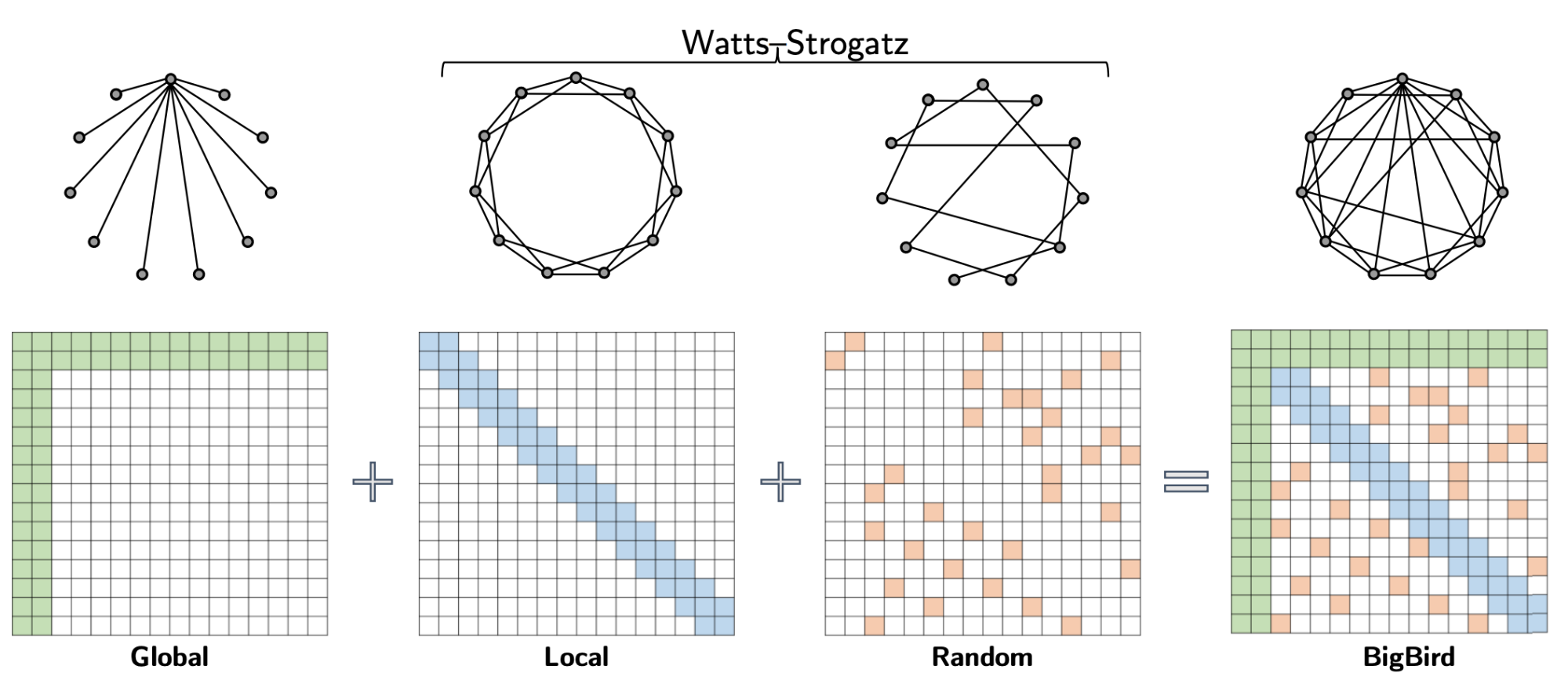 |
| The BigBird sparse attention model consists of global tokens that attend to all parts of an input sequence, local tokens, and a set of random tokens. Theoretically, this can be interpreted as adding a few global tokens on a Watts-Strogatz graph. |
The use of sparsity in models is clearly an approach with very high potential payoff in terms of computational efficiency, and we are only scratching the surface in terms of research ideas to be tried in this direction.
Each of these approaches for improved efficiency can be combined together so that equivalent-accuracy language models trained today in efficient data centers are ~100 times more energy efficient and produce ~650 times less CO2e emissions, compared to a baseline Transformer model trained using P100 GPUs in an average U.S. datacenter using an average U.S. energy mix. And this doesn’t even account for Google’s carbon-neutral, 100% renewable energy offsets. We’ll have a more detailed blog post analyzing the carbon emissions trends of NLP models soon.
Top
Trend 3: ML Is Becoming More Personally and Communally Beneficial
A host of new experiences are made possible as innovation in ML and silicon hardware (like the Google Tensor processor on the Pixel 6) enable mobile devices to be more capable of continuously and efficiently sensing their surrounding context and environment. These advances have improved accessibility and ease of use, while also boosting computational power, which is critical for popular features like mobile photography, live translation and more. Remarkably, recent technological advances also provide users with a more customized experience while strengthening privacy safeguards.
More people than ever rely on their phone cameras to record their daily lives and for artistic expression. The clever application of ML to computational photography has continued to advance the capabilities of phone cameras, making them easier to use, improving performance, and resulting in higher-quality images. Advances, such as improved HDR+, the ability to take pictures in very low light, better handling of portraits, and efforts to make cameras more inclusive so they work for all skin tones, yield better photos that are more true to the photographer’s vision and to their subjects. Such photos can be further improved using the powerful ML-based tools now available in Google Photos, like cinematic photos, noise and blur reduction, and the Magic Eraser.
 |
| HDR+ starts from a burst of full-resolution raw images, each underexposed by the same amount (left). The merged image has reduced noise and increased dynamic range, leading to a higher quality final result (right). |
In addition to using their phones for creative expression, many people rely on them to help communicate with others across languages and modalities in real-time using Live Translate in messaging apps and Live Caption for phone calls. Speech recognition accuracy has continued to make substantial improvements thanks to techniques like self-supervised learning and noisy student training, with marked improvements for accented speech, noisy conditions or environments with overlapping speech, and across many languages. Building on advances in text-to-speech synthesis, people can listen to web pages and articles using our Read Aloud technology on a growing number of platforms, making information more available across barriers of modality and languages. Live speech translations in the Google Translate app have become significantly better by stabilizing the translations that are generated on-the-fly, and high quality, robust and responsible direct speech-to-speech translation provides a much better user experience in communicating with people speaking a different language. New work on combining ML with traditional codec approaches in the Lyra speech codec and the more general SoundStream audio codec enables higher fidelity speech, music, and other sounds to be communicated reliably at much lower bitrate.
Everyday interactions are becoming much more natural with features like automatic call screening and ML agents that will wait on hold for you, thanks to advances in Duplex. Even short tasks that users may perform frequently have been improved with tools such as Smart Text Selection, which automatically selects entities like phone numbers or addresses for easy copy and pasting, and grammar correction as you type on Pixel 6 phones. In addition, Screen Attention prevents the phone screen from dimming when you are looking at it and improvements in gaze recognition are opening up new use cases for accessibility and for improved wellness and health. ML is also enabling new methods for ensuring the safety of people and communities. For example, Suspicious Message Alerts warn against possible phishing attacks and Safer Routing detects hard-braking events to suggest alternate routes.
 |
| Recent work demonstrates the ability of gaze recognition as an important biomarker of mental fatigue. |
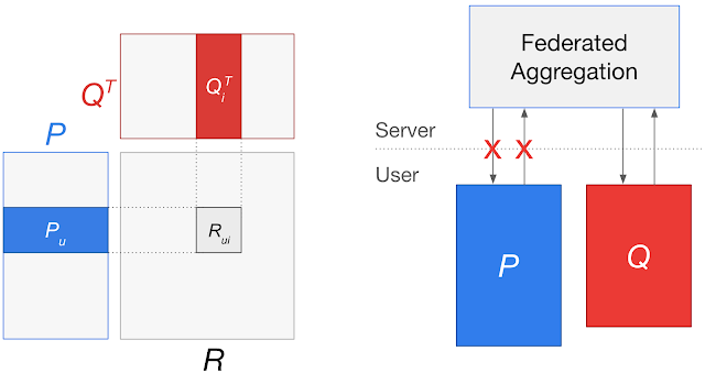
Given the potentially sensitive nature of the data that underlies these new capabilities, it is essential that they are designed to be private by default. Many of them run inside of Android’s Private Compute Core — an open source, secure environment isolated from the rest of the operating system. Android ensures that data processed in the Private Compute Core is not shared to any apps without the user taking an action. Android also prevents any feature inside the Private Compute Core from having direct access to the network. Instead, features communicate over a small set of open-source APIs to Private Compute Services, which strips out identifying information and makes use of privacy technologies, including federated learning, federated analytics, and private information retrieval, enabling learning while simultaneously ensuring privacy.
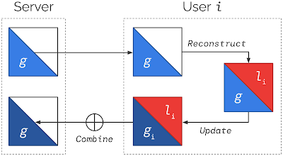 |
| Federated Reconstruction is a novel partially local federated learning technique in which models are partitioned into global and local parameters. For each round of Federated Reconstruction training: (1) The server sends the current global parameters g to each user i; (2) Each user i freezes g and reconstructs their local parameters li; (3) Each user i freezes li and updates g to produce gi; (4) Users’ gi are averaged to produce the global parameters for the next round. |
These technologies are critical to evolving next-generation computation and interaction paradigms, whereby personal or communal devices can both learn from and contribute to training a collective model of the world without compromising privacy. A federated unsupervised approach to privately learn the kinds of aforementioned general-purpose models with fine-tuning for a given task or context could unlock increasingly intelligent systems that are far more intuitive to interact with — more like a social entity than a machine. Broad and equitable access to these intelligent interfaces will only be possible with deep changes to our technology stacks, from the edge to the datacenter, so that they properly support neural computing.
Top
Trend 4: Growing Impact of ML in Science, Health and Sustainability
In recent years, we have seen an increasing impact of ML in the basic sciences, from physics to biology, with a number of exciting practical applications in related realms, such as renewable energy and medicine. Computer vision models have been deployed to address problems at both personal and global scales. They can assist physicians in their regular work, expand our understanding of neural physiology, and also provide better weather forecasts and streamline disaster relief efforts. Other types of ML models are proving critical in addressing climate change by discovering ways to reduce emissions and improving the output of alternative energy sources. Such models can even be leveraged as creative tools for artists! As ML becomes more robust, well-developed, and widely accessible, its potential for high-impact applications in a broad array of real-world domains continues to expand, helping to solve some of our most challenging problems.
Large-Scale Application of Computer Vision for New Insights
The advances in computer vision over the past decade have enabled computers to be used for a wide variety of tasks across different scientific domains. In neuroscience, automated reconstruction techniques can recover the neural connective structure of brain tissues from high resolution electron microscopy images of thin slices of brain tissue. In previous years, we have collaborated to create such resources for fruit fly, mouse, and songbird brains, but last year, we collaborated with the Lichtman Lab at Harvard University to analyze the largest sample of brain tissue imaged and reconstructed in this level of detail, in any species, and produced the first large-scale study of synaptic connectivity in the human cortex that spans multiple cell types across all layers of the cortex. The goal of this work is to produce a novel resource to assist neuroscientists in studying the stunning complexity of the human brain. The image below, for example, shows six neurons out of about 86 billion neurons in an adult human brain.
Computer vision technology also provides powerful tools to address challenges at much larger, even global, scales. A deep-learning–based approach to weather forecasting that uses satellite and radar imagery as inputs, combined with other atmospheric data, produces weather and precipitation forecasts that are more accurate than traditional physics-based models at forecasting times up to 12 hours. They can also produce updated forecasts much more quickly than traditional methods, which can be critical in times of extreme weather.
 |
| Comparison of 0.2 mm/hr precipitation on March 30, 2020 over Denver, Colorado. Left: Ground truth, source MRMS. Center: Probability map as predicted by MetNet-2. Right: Probability map as predicted by the physics-based HREF model. MetNet-2 is able to predict the onset of the storm earlier in the forecast than HREF as well as the storm’s starting location, whereas HREF misses the initiation location, but captures its growth phase well. |
Having an accurate record of building footprints is essential for a range of applications, from population estimation and urban planning to humanitarian response and environmental science. In many parts of the world, including much of Africa, this information wasn’t previously available, but new work shows that using computer vision techniques applied to satellite imagery can help identify building boundaries at continental scales. The results of this approach have been released in the Open Buildings dataset, a new open-access data resource that contains the locations and footprints of 516 million buildings with coverage across most of the African continent. We’ve also been able to use this unique dataset in our collaboration with the World Food Programme to provide fast damage assessment after natural disasters through application of ML.
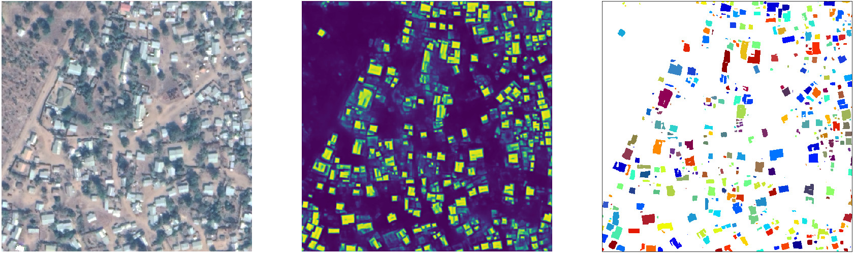 |
| Example of segmenting buildings in satellite imagery. Left: Source image; Center: Semantic segmentation, with each pixel assigned a confidence score that it is a building vs. non-building; Right: Instance segmentation, obtained by thresholding and grouping together connected components. |
A common theme across each of these cases is that ML models are able to perform specialized tasks efficiently and accurately based on analysis of available visual data, supporting high impact downstream tasks.
Automated Design Space Exploration
Another approach that has yielded excellent results across many fields is to allow an ML algorithm to explore and evaluate a problem’s design space for possible solutions in an automated way. In one application, a Transformer-based variational autoencoder learns to create aesthetically-pleasing and useful document layouts, and the same approach can be extended to explore possible furniture layouts. Another ML-driven approach automates the exploration of the huge design space of tweaks for computer game rules to improve playability and other attributes of a game, enabling human game designers to create enjoyable games more quickly.
 |
| A visualization of the Variational Transformer Network (VTN) model, which is able to extract meaningful relationships between the layout elements (paragraphs, tables, images, etc.) in order to generate realistic synthetic documents (e.g., with better alignment and margins). |
Other ML algorithms have been used to evaluate the design space of computer architectural decisions for ML accelerator chips themselves. We’ve also shown that ML can be used to quickly create chip placements for ASIC designs that are better than layouts generated by human experts and can be generated in a matter of hours instead of weeks. This reduces the fixed engineering costs of chips and lowers the barrier to quickly creating specialized hardware for different applications. We’ve successfully used this automated placement approach in the design of our upcoming TPU-v5 chip.
Such exploratory ML approaches have also been applied to materials discovery. In a collaboration between Google Research and Caltech, several ML models, combined with a modified inkjet printer and a custom-built microscope, were able to rapidly search over hundreds of thousands of possible materials to hone in on 51 previously uncharacterized three-metal oxide materials with promising properties for applications in areas like battery technology and electrolysis of water.
These automated design space exploration approaches can help accelerate many scientific fields, especially when the entire experimental loop of generating the experiment and evaluating the result can all be done in an automated or mostly-automated manner. I expect to see this approach applied to good effect in many more areas in the coming years.
Application to Health
In addition to advancing basic science, ML can also drive advances in medicine and human health more broadly. The idea of leveraging advances in computer science in health is nothing new — in fact some of my own early experiences were in developing software to help analyze epidemiological data. But ML opens new doors, raises new opportunities, and yes, poses new challenges.
Take for example the field of genomics. Computing has been important to genomics since its inception, but ML adds new capabilities and disrupts old paradigms. When Google researchers began working in this area, the idea of using deep learning to help infer genetic variants from sequencer output was considered far-fetched by many experts. Today, this ML approach is considered state-of-the-art. But the future holds an even more important role for ML — genomics companies are developing new sequencing instruments that are more accurate and faster, but also present new inference challenges. Our release of open-source software DeepConsensus and, in collaboration with UCSC, PEPPER-DeepVariant, supports these new instruments with cutting-edge informatics. We hope that more rapid sequencing can lead to near term applicability with impact for real patients.
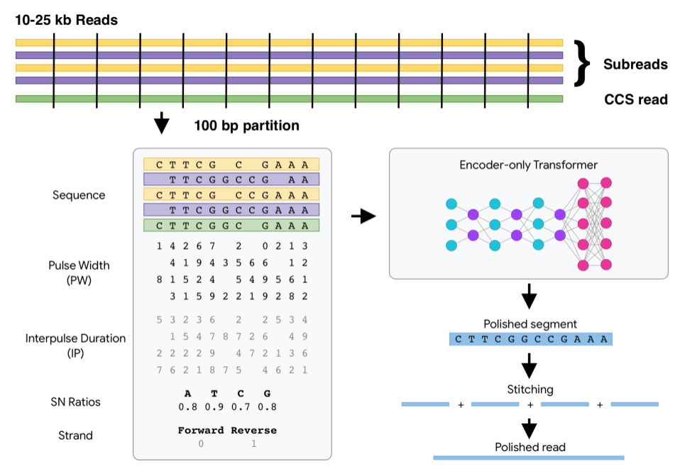 |
| A schematic of the Transformer architecture for DeepConsensus, which corrects sequencing errors to improve yield and correctness. |
There are other opportunities to use ML to accelerate our use of genomic information for personalized health outside of processing the sequencer data. Large biobanks of extensively phenotyped and sequenced individuals can revolutionize how we understand and manage genetic predisposition to disease. Our ML-based phenotyping method improves the scalability of converting large imaging and text datasets into phenotypes usable for genetic association studies, and our DeepNull method better leverages large phenotypic data for genetic discovery. We are happy to release both as open-source methods for the scientific community.
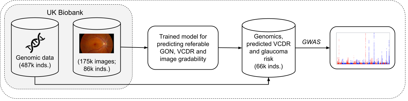 |
| The process for generating large-scale quantification of anatomical and disease traits for combination with genomic data in Biobanks. |
Just as ML helps us see hidden characteristics of genomics data, it can help us discover new information and glean new insights from other health data types as well. Diagnosis of disease is often about identifying a pattern, quantifying a correlation, or recognizing a new instance of a larger class — all tasks at which ML excels. Google researchers have used ML to tackle a wide range of such problems, but perhaps none of these has progressed farther than the applications of ML to medical imaging.
In fact, Google’s 2016 paper describing the application of deep learning to the screening for diabetic retinopathy, was selected by the editors of the Journal of the American Medical Association (JAMA) as one of the top 10 most influential papers of the decade — not just the most influential papers on ML and health, the most influential JAMA papers of the decade overall. But the strength of our research doesn’t end at contributions to the literature, but extends to our ability to build systems operating in the real world. Through our global network of deployment partners, this same program has helped screen tens of thousands of patients in India, Thailand, Germany and France who might otherwise have been untested for this vision-threatening disease.
We expect to see this same pattern of assistive ML systems deployed to improve breast cancer screening, detect lung cancer, accelerate radiotherapy treatments for cancer, flag abnormal X-rays, and stage prostate cancer biopsies. Each domain presents new opportunities to be helpful. ML-assisted colonoscopy procedures are a particularly interesting example of going beyond the basics. Colonoscopies are not just used to diagnose colon cancer — the removal of polyps during the procedure are the front line of halting disease progression and preventing serious illness. In this domain we’ve demonstrated that ML can help ensure doctors don’t miss polyps, can help detect elusive polyps, and can add new dimensions of quality assurance, like coverage mapping through the application of simultaneous localization and mapping techniques. In collaboration with Shaare Zedek Medical Center in Jerusalem, we’ve shown these systems can work in real time, detecting an average of one polyp per procedure that would have otherwise been missed, with fewer than four false alarms per procedure.
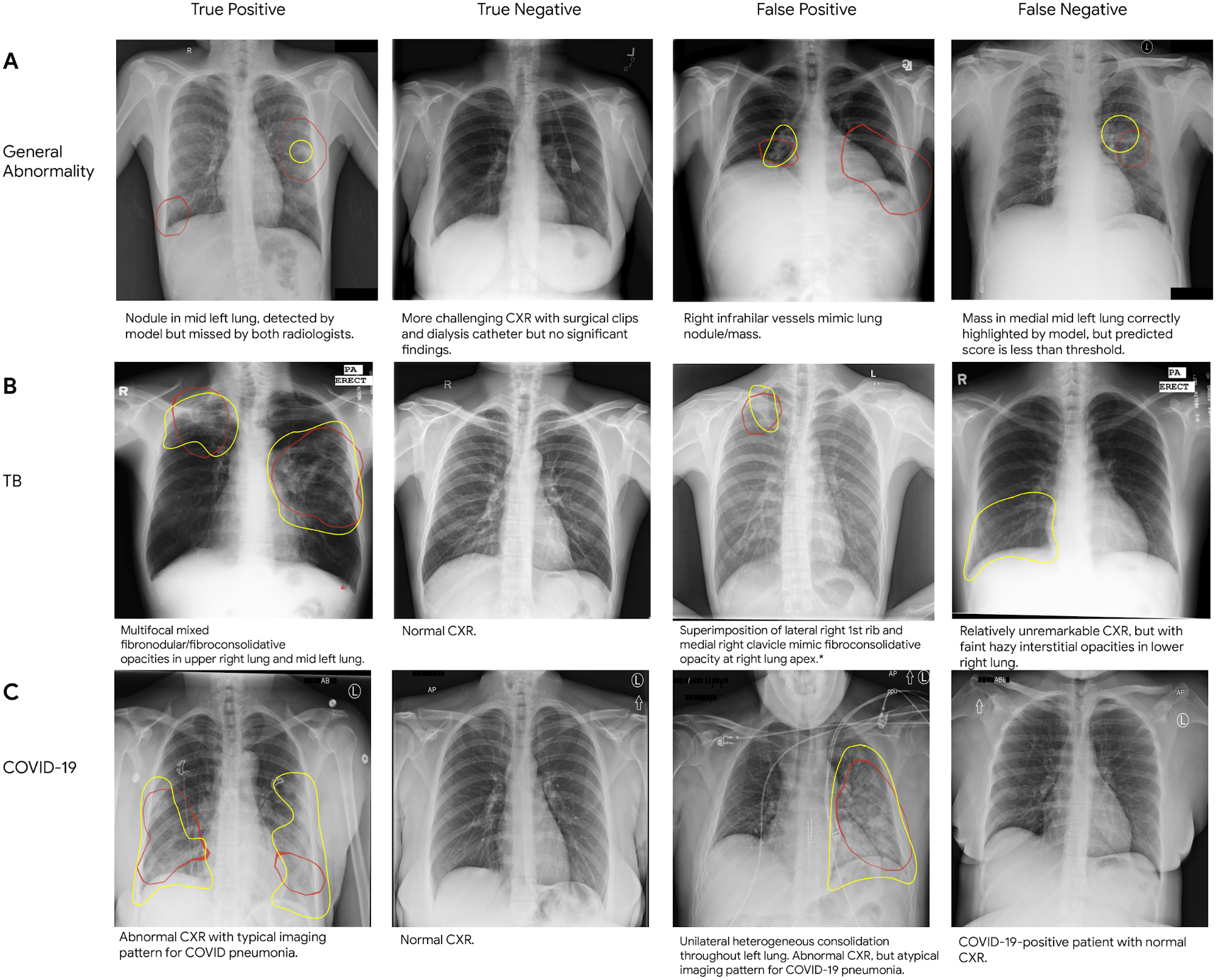 |
| Sample chest X-rays (CXR) of true and false positives, and true and false negatives for (A) general abnormalities, (B) tuberculosis, and (C) COVID-19. On each CXR, red outlines indicate areas on which the model focused to identify abnormalities (i.e., the class activation map), and yellow outlines refer to regions of interest identified by a radiologist. |
Another ambitious healthcare initiative, Care Studio, uses state-of-the-art ML and advanced NLP techniques to analyze structured data and medical notes, presenting clinicians with the most relevant information at the right time — ultimately helping them deliver more proactive and accurate care.
As important as ML may be to expanding access and improving accuracy in the clinical setting, we see a new equally important trend emerging: ML applied to help people in their daily health and well-being. Our everyday devices have powerful sensors that can help democratize health metrics and information so people can make more informed decisions about their health. We’ve already seen launches that enable a smartphone camera to assess heart rate and respiratory rate to help users without additional hardware, and Nest Hub devices that support contactless sleep sensing and allow users to better understand their nighttime wellness. We’ve seen that we can, on the one hand, significantly improve speech recognition quality for disordered speech in our own ASR systems, and on the other, use ML to help recreate the voice of those with speech impairments, empowering them to communicate in their own voice. ML enabled smartphones that help people better research emerging skin conditions or help those with limited vision go for a jog, seem to be just around the corner. These opportunities offer a future too bright to ignore.
 |
| The custom ML model for contactless sleep sensing efficiently processes a continuous stream of 3D radar tensors (summarizing activity over a range of distances, frequencies, and time) to automatically compute probabilities for the likelihood of user presence and wakefulness (awake or asleep). |
ML Applications for the Climate Crisis
Another realm of paramount importance is climate change, which is an incredibly urgent threat for humanity. We need to all work together to bend the curve of harmful emissions to ensure a safe and prosperous future. Better information about the climate impact of different choices can help us tackle this challenge in a number of different ways.
To this end, we recently rolled out eco-friendly routing in Google Maps, which we estimate will save about 1 million tons of CO2 emissions per year (the equivalent of removing more than 200,000 cars from the road). A recent case study shows that using Google Maps directions in Salt Lake City results in both faster and more emissions-friendly routing, which saves 1.7% of CO2 emissions and 6.5% travel time. In addition, making our Maps products smarter about electric vehicles can help alleviate range anxiety, encouraging people to switch to emissions-free vehicles. We are also working with multiple municipalities around the world to use aggregated historical traffic data to help suggest improved traffic light timing settings, with an early pilot study in Israel and Brazil showing a 10-20% reduction in fuel consumption and delay time at the examined intersections.
 |
| With eco-friendly routing, Google Maps will show you the fastest route and the one that’s most fuel-efficient — so you can choose whichever one works best for you. |
On a longer time scale, fusion holds promise as a game-changing renewable energy source. In a long-standing collaboration with TAE Technologies, we have used ML to help maintain stable plasmas in their fusion reactor by suggesting settings of the more than 1000 relevant control parameters. With our collaboration, TAE achieved their major goals for their Norman reactor, which brings us a step closer to the goal of breakeven fusion. The machine maintains a stable plasma at 30 million Kelvin (don’t touch!) for 30 milliseconds, which is the extent of available power to its systems. They have completed a design for an even more powerful machine, which they hope will demonstrate the conditions necessary for breakeven fusion before the end of the decade.
We’re also expanding our efforts to address wildfires and floods, which are becoming more common (like millions of Californians, I’m having to adapt to having a regular “fire season”). Last year, we launched a wildfire boundary map powered by satellite data to help people in the U.S. easily understand the approximate size and location of a fire — right from their device. Building on this, we’re now bringing all of Google’s wildfire information together and launching it globally with a new layer on Google Maps. We have been applying graph optimization algorithms to help optimize fire evacuation routes to help keep people safe in the presence of rapidly advancing fires. In 2021, our Flood Forecasting Initiative expanded its operational warning systems to cover 360 million people, and sent more than 115 million notifications directly to the mobile devices of people at risk from flooding, more than triple our outreach in the previous year. We also deployed our LSTM-based forecast models and the new Manifold inundation model in real-world systems for the first time, and shared a detailed description of all components of our systems.
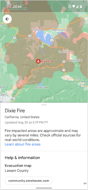 |
| The wildfire layer in Google Maps provides people with critical, up-to-date information in an emergency. |
We’re also working hard on our own set of sustainability initiatives. Google was the first major company to become carbon neutral in 2007. We were also the first major company to match our energy use with 100 percent renewable energy in 2017. We operate the cleanest global cloud in the industry, and we’re the world’s largest corporate purchaser of renewable energy. Further, in 2020 we became the first major company to make a commitment to operate on 24/7 carbon-free energy in all our data centers and campuses worldwide. This is far more challenging than the traditional approach of matching energy usage with renewable energy, but we’re working to get this done by 2030. Carbon emission from ML model training is a concern for the ML community, and we have shown that making good choices about model architecture, datacenter, and ML accelerator type can reduce the carbon footprint of training by ~100-1000x.
Top
Trend 5: Deeper and Broader Understanding of ML
As ML is used more broadly across technology products and society more generally, it is imperative that we continue to develop new techniques to ensure that it is applied fairly and equitably, and that it benefits all people and not just select subsets. This is a major focus for our Responsible AI and Human-Centered Technology research group and an area in which we conduct research on a variety of responsibility-related topics.
One area of focus is recommendation systems that are based on user activity in online products. Because these recommendation systems are often composed of multiple distinct components, understanding their fairness properties often requires insight into individual components as well as how the individual components behave when combined together. Recent work has helped to better understand these relationships, revealing ways to improve the fairness of both individual components and the overall recommendation system. In addition, when learning from implicit user activity, it is also important for recommendation systems to learn in an unbiased manner, since the straightforward approach of learning from items that were shown to previous users exhibits well-known forms of bias. Without correcting for such biases, for example, items that were shown in more prominent positions to users tend to get recommended to future users more often.
As in recommendation systems, surrounding context is important in machine translation. Because most machine translation systems translate individual sentences in isolation, without additional surrounding context, they can often reinforce biases related to gender, age or other areas. In an effort to address some of these issues, we have a long-standing line of research on reducing gender bias in our translation systems, and to help the entire translation community, last year we released a dataset to study gender bias in translation based on translations of Wikipedia biographies.
Another common problem in deploying machine learning models is distributional shift: if the statistical distribution of data on which the model was trained is not the same as that of the data the model is given as input, the model’s behavior can sometimes be unpredictable. In recent work, we employ the Deep Bootstrap framework to compare the real world, where there is finite training data, to an “ideal world”, where there is infinite data. Better understanding of how a model behaves in these two regimes (real vs. ideal) can help us develop models that generalize better to new settings and exhibit less bias towards fixed training datasets.
Although work on ML algorithms and model development gets significant attention, data collection and dataset curation often gets less. But this is an important area, because the data on which an ML model is trained can be a potential source of bias and fairness issues in downstream applications. Analyzing such data cascades in ML can help identify the many places in the lifecycle of an ML project that can have substantial influence on the outcomes. This research on data cascades has led to evidence-backed guidelines for data collection and evaluation in the revised PAIR Guidebook, aimed at ML developers and designers.
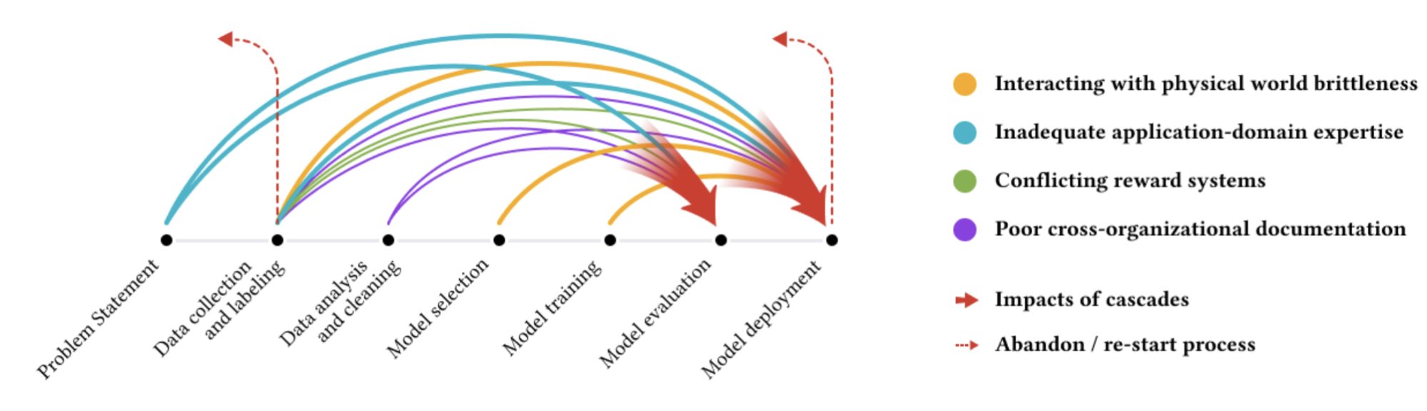 |
| Arrows of different color indicate various types of data cascades, each of which typically originate upstream, compound over the ML development process, and manifest downstream. |
The general goal of better understanding data is an important part of ML research. One thing that can help is finding and investigating anomalous data. We have developed methods to better understand the influence that particular training examples can have on an ML model, since mislabeled data or other similar issues can have outsized impact on the overall model behavior. We have also built the Know Your Data tool to help ML researchers and practitioners better understand properties of their datasets, and last year we created a case study of how to use the Know Your Data tool to explore issues like gender bias and age bias in a dataset.
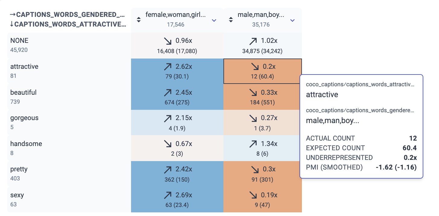 |
| A screenshot from Know Your Data showing the relationship between words that describe attractiveness and gendered words. For example, “attractive” and “male/man/boy” co-occur 12 times, but we expect ~60 times by chance (the ratio is 0.2x). On the other hand, “attractive” and “female/woman/girl” co-occur 2.62 times more than chance. |
Understanding dynamics of benchmark dataset usage is also important, given the central role they play in the organization of ML as a field. Although studies of individual datasets have become increasingly common, the dynamics of dataset usage across the field have remained underexplored. In recent work, we published the first large scale empirical analysis of dynamics of dataset creation, adoption, and reuse. This work offers insights into pathways to enable more rigorous evaluations, as well as more equitable and socially informed research.
Creating public datasets that are more inclusive and less biased is an important way to help improve the field of ML for everyone. In 2016, we released the Open Images dataset, a collection of ~9 million images annotated with image labels spanning thousands of object categories and bounding box annotations for 600 classes. Last year, we introduced the More Inclusive Annotations for People (MIAP) dataset in the Open Images Extended collection. The collection contains more complete bounding box annotations for the person class hierarchy, and each annotation is labeled with fairness-related attributes, including perceived gender presentation and perceived age range. With the increasing focus on reducing unfair bias as part of responsible AI research, we hope these annotations will encourage researchers already leveraging the Open Images dataset to incorporate fairness analysis in their research.
Because we also know that our teams are not the only ones creating datasets that can improve machine learning, we have built Dataset Search to help users discover new and useful datasets, wherever they might be on the Web.
Tackling various forms of abusive behavior online, such as toxic language, hate speech, and misinformation, is a core priority for Google. Being able to detect such forms of abuse reliably, efficiently, and at scale is of critical importance both to ensure that our platforms are safe and also to avoid the risk of reproducing such negative traits through language technologies that learn from online discourse in an unsupervised fashion. Google has pioneered work in this space through the Perspective API tool, but the nuances involved in detecting toxicity at scale remains a complex problem. In recent work, in collaboration with various academic partners, we introduced a comprehensive taxonomy to reason about the changing landscape of online hate and harassment. We also investigated how to detect covert forms of toxicity, such as microaggressions, that are often ignored in online abuse interventions, studied how conventional approaches to deal with disagreements in data annotations of such subjective concepts might marginalize minority perspectives, and proposed a new disaggregated modeling approach that uses a multi-task framework to tackle this issue. Furthermore, through qualitative research and network-level content analysis, Google’s Jigsaw team, in collaboration with researchers at George Washington University, studied how hate clusters spread disinformation across social media platforms.
Another potential concern is that ML language understanding and generation models can sometimes also produce results that are not properly supported by evidence. To confront this problem in question answering, summarization, and dialog, we developed a new framework for measuring whether results can be attributed to specific sources. We released annotation guidelines and demonstrated that they can be reliably used in evaluating candidate models.
Interactive analysis and debugging of models remains key to responsible use of ML. We have updated our Language Interpretability Tool with new capabilities and techniques to advance this line of work, including support for image and tabular data, a variety of features carried over from our previous work on the What-If Tool, and built-in support for fairness analysis through the technique of Testing with Concept Activation Vectors. Interpretability and explainability of ML systems more generally is also a key part of our Responsible AI vision; in collaboration with DeepMind, we made headway in understanding the acquisition of human chess concepts in the self-trained AlphaZero chess system.
We are also working hard to broaden the perspective of Responsible AI beyond western contexts. Our recent research examines how various assumptions of conventional algorithmic fairness frameworks based on Western institutions and infrastructures may fail in non-Western contexts and offers a pathway for recontextualizing fairness research in India along several directions. We are actively conducting survey research across several continents to better understand perceptions of and preferences regarding AI. Western framing of algorithmic fairness research tends to focus on only a handful of attributes, thus biases concerning non-Western contexts are largely ignored and empirically under-studied. To address this gap, in collaboration with the University of Michigan, we developed a weakly supervised method to robustly detect lexical biases in broader geo-cultural contexts in NLP models that reflect human judgments of offensive and inoffensive language in those geographic contexts.
Furthermore, we have explored applications of ML to contexts valued in the Global South, including developing a proposal for farmer-centered ML research. Through this work, we hope to encourage the field to be thoughtful about how to bring ML-enabled solutions to smallholder farmers in ways that will improve their lives and their communities.
Involving community stakeholders at all stages of the ML pipeline is key to our efforts to develop and deploy ML responsibly and keep us focused on tackling the problems that matter most. In this vein, we held a Health Equity Research Summit among external faculty, non-profit organization leads, government and NGO representatives, and other subject matter experts to discuss how to bring more equity into the entire ML ecosystem, from the way we approach problem-solving to how we assess the impact of our efforts.
Community-based research methods have also informed our approach to designing for digital wellbeing and addressing racial equity issues in ML systems, including improving our understanding of the experience of Black Americans using ASR systems. We are also listening to the public more broadly to learn how sociotechnical ML systems could help during major life events, such as by supporting family caregiving.
As ML models become more capable and have impact in many domains, the protection of the private information used in ML continues to be an important focus for research. Along these lines, some of our recent work addresses privacy in large models, both highlighting that training data can sometimes be extracted from large models and pointing to how privacy can be achieved in large models, e.g., as in differentially private BERT. In addition to the work on federated learning and analytics, mentioned above, we have also been enhancing our toolbox with other principled and practical ML techniques for ensuring differential privacy, for example private clustering, private personalization, private matrix completion, private weighted sampling, private quantiles, private robust learning of halfspaces, and in general, sample-efficient private PAC learning. Moreover, we have been expanding the set of privacy notions that can be tailored to different applications and threat models, including label privacy and user versus item level privacy.
Top
Datasets
Recognizing the value of open datasets to the general advancement of ML and related fields of research, we continue to grow our collection of open source datasets and resources and expand our global index of open datasets in Google Dataset Search. This year, we have released a number of datasets and tools across a range of research areas:
| Datasets & Tools |
Description |
| AIST++ |
3D keypoints with corresponding images for dance motions covering 10 dance genres |
| AutoFlow |
40k image pairs with ground truth optical flow |
| C4_200M |
A 200 million sentence synthetic dataset for grammatical error correction |
| CIFAR-5M |
Dataset of ~6 million synthetic CIFAR-10–like images (RGB 32 x 32 pix) |
| Crisscrossed Captions |
Set of semantic similarity ratings for the MS-COCO dataset |
| Disfl-QA |
Dataset of contextual disfluencies for information seeking |
| Distilled Datasets |
Distilled datasets from CIFAR-10, CIFAR-100, MNIST, Fashion-MNIST, and SVHN |
| EvolvingRL |
1000 top performing RL algorithms discovered through algorithm evolution |
| GoEmotions |
A human-annotated dataset of 58k Reddit comments labeled with 27 emotion categories |
| H01 Dataset |
1.4 petabyte browsable reconstruction of the human cortex |
| Know Your Data |
Tool for understanding biases in a dataset |
| Lens Flare |
5000 high-quality RGB images of typical lens flare |
| More Inclusive Annotations for People (MIAP) |
Improved bounding box annotations for a subset of the person class in the Open Images dataset |
| Mostly Basic Python Problems |
1000 Python programming problems, incl. task description, code solution & test cases |
| NIH ChestX-ray14 dataset labels |
Expert labels for a subset of the NIH ChestX-ray14 dataset |
| Open Buildings |
Locations and footprints of 516 million buildings with coverage across most of Africa |
| Optical Polarization from Curie |
5GB of optical polarization data from the Curie submarine cable |
| Readability Scroll |
Scroll interactions of ~600 participants reading texts from the OneStopEnglish corpus |
| RLDS |
Tools to store, retrieve & manipulate episodic data for reinforcement learning |
| Room-Across-Room (RxR) |
Multilingual dataset for vision-and-language navigation in English, Hindi and Telugu |
| Soft Attributes |
~6k sets of movie titles annotated with single English soft attributes |
| TimeDial |
Dataset of multiple choice span-filling tasks for temporal commonsense reasoning in dialog |
| ToTTo |
English table-to-text generation dataset with a controlled text generation task |
| Translated Wikipedia Biographies |
Dataset for analysis of common gender errors in NMT for English, Spanish and German |
| UI Understanding Data for UIBert |
Datasets for two UI understanding tasks, AppSim & RefExp |
| WikiFact |
Wikipedia & WikiData–based dataset to train relationship classifiers and fact extraction models |
| WIT |
Wikipedia-based Image Text dataset for multimodal multilingual ML |
Research Community Interaction
To realize our goal for a more robust and comprehensive understanding of ML and related technologies, we actively engage with the broader research community. In 2021, we published over 750 papers, nearly 600 of which were presented at leading research conferences. Google Research sponsored over 150 conferences, and Google researchers contributed directly by serving on program committees and organizing workshops, tutorials and numerous other activities aimed at collectively advancing the field. To learn more about our contributions to some of the larger research conferences this year, please see our recent conference blog posts. In addition, we hosted 19 virtual workshops (like the 2021 Quantum Summer Symposium), which allowed us to further engage with the academic community by generating new ideas and directions for the research field and advancing research initiatives.
In 2021, Google Research also directly supported external research with $59M in funding, including $23M through Research programs to faculty and students, and $20M in university partnerships and outreach. This past year, we introduced new funding and collaboration programs that support academics all over the world who are doing high impact research. We funded 86 early career faculty through our Research Scholar Program to support general advancements in science, and funded 34 faculty through our Award for Inclusion Research Program who are doing research in areas like accessibility, algorithmic fairness, higher education and collaboration, and participatory ML. In addition to the research we are funding, we welcomed 85 faculty and post-docs, globally, through our Visiting Researcher program, to come to Google and partner with us on exciting ideas and shared research challenges. We also selected a group of 74 incredibly talented PhD student researchers to receive Google PhD Fellowships and mentorship as they conduct their research.
As part of our ongoing racial equity commitments, making computer science (CS) research more inclusive continues to be a top priority for us. In 2021, we continued expanding our efforts to increase the diversity of Ph.D. graduates in computing. For example, the CS Research Mentorship Program (CSRMP), an initiative by Google Research to support students from historically marginalized groups (HMGs) in computing research pathways, graduated 590 mentees, 83% of whom self-identified as part of an HMG, who were supported by 194 Google mentors — our largest group to date! In October, we welcomed 35 institutions globally leading the way to engage 3,400+ students in computing research as part of the 2021 exploreCSR cohort. Since 2018, this program has provided faculty with funding, community, evaluation and connections to Google researchers in order to introduce students from HMGs to the world of CS research. We are excited to expand this program to more international locations in 2022.
We also continued our efforts to fund and partner with organizations to develop and support new pathways and approaches to broadening participation in computing research at scale. From working with alliances like the Computing Alliance of Hispanic-Serving Institutions (CAHSI) and CMD-IT Diversifying LEAdership in the Professoriate (LEAP) Alliance to partnering with university initiatives like UMBC’s Meyerhoff Scholars, Cornell University’s CSMore, Northeastern University’s Center for Inclusive Computing, and MIT’s MEnTorEd Opportunities in Research (METEOR), we are taking a community-based approach to materially increase the representation of marginalized groups in computing research.
Other Work
In writing these retrospectives, I try to focus on new research work that has happened (mostly) in the past year while also looking ahead. In past years’ retrospectives, I’ve tried to be more comprehensive, but this time I thought it could be more interesting to focus on just a few themes. We’ve also done great work in many other research areas that don’t fit neatly into these themes. If you’re interested, I encourage you to check out our research publications by area below or by year (and if you’re interested in quantum computing, our Quantum team recently wrote a retrospective of their work in 2021):
Conclusion
Research is often a multi-year journey to real-world impact. Early stage research work that happened a few years ago is now having a dramatic impact on Google’s products and across the world. Investments in ML hardware accelerators like TPUs and in software frameworks like TensorFlow and JAX have borne fruit. ML models are increasingly prevalent in many different products and features at Google because their power and ease of expression streamline experimentation and productionization of ML models in performance-critical environments. Research into model architectures to create Seq2Seq, Inception, EfficientNet, and Transformer or algorithmic research like batch normalization and distillation is driving progress in the fields of language understanding, vision, speech, and others. Basic capabilities like better language and visual understanding and speech recognition can be transformational, and as a result, these sorts of models are widely deployed for a wide variety of problems in many of our products including Search, Assistant, Ads, Cloud, Gmail, Maps, YouTube, Workspace, Android, Pixel, Nest, and Translate.
These are truly exciting times in machine learning and computer science. Continued improvement in computers’ ability to understand and interact with the world around them through language, vision, and sound opens up entire new frontiers of how computers can help people accomplish things in the world. The many examples of progress along the five themes outlined in this post are waypoints in a long-term journey!
Acknowledgements
Thanks to Alison Carroll, Alison Lentz, Andrew Carroll, Andrew Tomkins, Avinatan Hassidim, Azalia Mirhoseini, Barak Turovsky, Been Kim, Blaise Aguera y Arcas, Brennan Saeta, Brian Rakowski, Charina Chou, Christian Howard, Claire Cui, Corinna Cortes, Courtney Heldreth, David Patterson, Dipanjan Das, Ed Chi, Eli Collins, Emily Denton, Fernando Pereira, Genevieve Park, Greg Corrado, Ian Tenney, Iz Conroy, James Wexler, Jason Freidenfelds, John Platt, Katherine Chou, Kathy Meier-Hellstern, Kyle Vandenberg, Lauren Wilcox, Lizzie Dorfman, Marian Croak, Martin Abadi, Matthew Flegal, Meredith Morris, Natasha Noy, Negar Saei, Neha Arora, Paul Muret, Paul Natsev, Quoc Le, Ravi Kumar, Rina Panigrahy, Sanjiv Kumar, Sella Nevo, Slav Petrov, Sreenivas Gollapudi, Tom Duerig, Tom Small, Vidhya Navalpakkam, Vincent Vanhoucke, Vinodkumar Prabhakaran, Viren Jain, Yonghui Wu, Yossi Matias, and Zoubin Ghahramani for helpful feedback and contributions to this post, and to the entire Research and Health communities at Google for everyone’s contributions towards this work.


%E2%80%93Weddell_seal_(Leptonychotes_weddellii)_03.jpg)