
Sparklyr 1.7 delivers much-anticipated improvements, including R interfaces for image and binary data sources, several new spark_apply() capabilities, and better integration with sparklyr extensions.
Category: Offsites
Stuff I find valuable at key websites
Categories
CodeReading – 4. Python Code Style
Code Reading은 잘 작성되어 있는 프레임워크, 라이브러리, 툴킷 등의 다양한 프로젝트의 내부를 살펴보는 시리즈 입니다. 프로젝트의 아키텍처, 디자인철학이나 코드 스타일 등을 살펴보며, 구체적으로 하나하나 살펴보는 것이 아닌 전반적이면서 간단하게 살펴봅니다.
이번 포스트에서는 프로젝트는 아니지만, 코드 자체와 관련이 깊은 Python 언어의 코드 스타일에 대해서 알아봅니다.
Series.
- CodeReading – 1. PyTorch
- CodeReading – 2. Flask
- CodeReading – 3. ABC
- CodeReading – 4. Python Code Style
Code Style의 중요성
코드스타일이 의미하는 것은 무엇이고, 왜 필요할까요?
코드스타일은 코드 가독성을 위해서 네이밍, 라인수, Indentation 등의 코드의 형식을 맞추는 것을 의미합니다. 이 활동은 특히 ‘협업’에 중점두고 있습니다. 즉 개인이 아닌 팀으로 일하는 경우에 사용하는 하나의 룰 혹은 가이드입니다.
이 Code Reading 시리즈에서 코드를 읽고 있는 것처럼, 코드는 기계 뿐만 아니라 사람들에게도 읽히게 됩니다. 특히 가장 많이 보게 되는 코드는 같이 협업을 하는 동료의 코드일 것 입니다. 이렇게 읽어야 하는 코드가 개인의 코드스타일에 따라서 작성되어 있다면 어떨까요? 스타일에 따라서 다르겠지만, 기본적으로 코드를 해석하는데 시간이 더 걸리게 될 것입니다. 하지만 팀 내부적으로 코드 스타일을 맞춰놓았다면, 훨씬 빠르게 로직을 이해할 수 있고 새롭게 기능을 추가하거나, 코드 리뷰를 하는 등의 다양한 활동을 조금 더 쉽게 진행할 수 있을 것 입니다.
이렇게 명확한 장점을 가지고 있는 코드스타일을 도입하는데 있어서, 한가지 주의할 점이 있습니다. 코드 스타일을 지원하는 다양한 툴이 있기도 하고, 회사마다 스타일 가이드가 있습니다. 즉 누군가에게 조금 더 선호되는 스타일이 있을 수 있지만, 딱 ‘이 스타일이 정답이다’ 라고 말할 수 없는 논술 문제에 가깝습니다. 그래서 팀 내부적으로 의논을 통해, 우리 팀에 맞는 스타일을 모두의 동의하에 정의하고 서로 맞춰나가는 것이 가장 중요합니다.
그렇다면 Pyhon Code Style에 대해서 조금 더 자세히 알아볼까요?
PEP8
Python 언어의 코드 스타일의 가장 기본이 되는 것은 PEP8 입니다. PEP(Python Enhance Proposal)은 공식적으로 운영되고 있는 개선 제안서로서, 그 중에서 PEP8 은 Style Guide for Python Code 이라는 제목으로 작성이 되어있습니다.
여기에는 다음과 같은 가이드들이 작성되어 있습니다. 간략하게 다뤄보면 다음과 같습니다.
- Indentation
# Correct:
# Aligned with opening delimiter.
foo = long_function_name(var_one, var_two,
                         var_three, var_four)

# Add 4 spaces (an extra level of indentation) to distinguish arguments from the rest.
def long_function_name(
        var_one, var_two, var_three,
        var_four):
    print(var_one)

# -------------------------
# Wrong:
# Arguments on first line forbidden when not using vertical alignment.
foo = long_function_name(var_one, var_two,
    var_three, var_four)

# Further indentation required as indentation is not distinguishable.
def long_function_name(
    var_one, var_two, var_three,
    var_four):
    print(var_one)
indentation의 경우, 함수의 arguments 들이 명확히 구별되도록 가이드하고 있습니다.
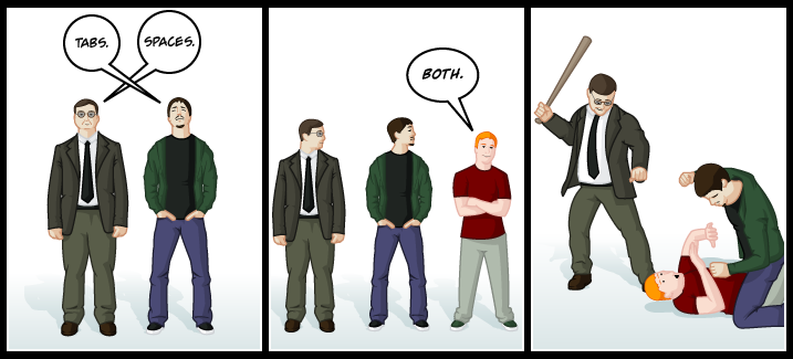
- Tabs vs Spaces
PEP8에서는 Space를 써야한다고 이야기하고 있고, 두가지를 혼합해서 사용하는 것을 금지하고 있습니다! (이 포스트 시작에 있는 그림과 연결되죠)
- 권장사항
아래와 같이 empty sequence 는 False 인 것을 이용해서, length를 기반으로 체크하지 않도록 권장하기도 합니다.
# Correct:
if not seq:
if seq:

# Wrong:
if len(seq):
if not len(seq):
가장 기본이 되는 스타일 가이드이기 때문에 전체를 한번 읽어보실 것을 추천드립니다. 대부분의 내용은 지금도 사용되고 있습니다. 다만, PEP8이 제안될 당시와 비교했을 때 개발 환경은 많이 달라졌습니다. 작은 모니터에서 다양한 크기의 모니터를 여러개 연결해서 개발을 하는 것이 흔해진 상황이죠. 그래서 Maximum Line Length의 경우에는 의견이 분분하기도 합니다. 모든 행을 79자 제한으로 제안되었지만, 더 길게 셋팅을 하는 경우도 흔하게 찾아볼 수 있습니다.
Tools
코드스타일에 관련한 도구들은 위의 PEP8을 기본으로 지원하면서 환경셋팅을 통해서 원하는대로 수정할 수 있도록 되어있습니다. 여러가지 도구들이 있지만, 최근에 가장 많이 사용하고 있는 black과 isort 두가지를 대표적으로 소개해드려고 합니다.
black
The Uncompromising Code Formatter
black은 비교적 최근(2018년)에 개발된 오픈소스로 정해진 코드의 규격에 맞춰서 정리해주는 Code Formatter 입니다. black의 가장 큰 특징은 바로 ‘타협하지 않는’ 입니다. 타협하지 않는 부분은 바로 PEP8 에서 커버하지 않고 있는, 사람마다 각각 스타일이 다른 부분입니다. 그래서 black의 공식 문서에서도 PEP을 준수하는 엄격한 하위집단이라고 이야기 하고 있습니다.
그러면 black에서 추구하는 코드 스타일에 대해서 간단하게 살펴보겠습니다.
- Maximum Line Length : 88 (80 에서 10% 늘어난 값)
- 줄 바꿈 방식
# [1] in:
ImportantClass.important_method(exc, limit, lookup_lines, capture_locals, extra_argument)

# [1] out:
ImportantClass.important_method(
    exc, limit, lookup_lines, capture_locals, extra_argument
)

# [2] in:
def very_important_function(template: str, *variables, file: os.PathLike, engine: str, header: bool = True, debug: bool = False):
    """Applies `variables` to the `template` and writes to `file`."""
    with open(file, 'w') as f:
        ...

# [2] out:
def very_important_function(
    template: str,
    *variables,
    file: os.PathLike,
    engine: str,
    header: bool = True,
    debug: bool = False,
):
    """Applies `variables` to the `template` and writes to `file`."""
    with open(file, "w") as f:
        ...

# [3] in:
if some_long_rule1
  and some_long_rule2:
    ...

# [3] out:
if (
    some_long_rule1
    and some_long_rule2
):
    ...
줄 길이에 따라서 위와 같이, 들여쓰기[1]가 되거나 파라미터가 더욱 많은 경우에는 하나하나 새로운 줄[2]에 위치하게 됩니다. 그리고 문장 길이를 맞추기 위해서 사용하는 백슬래시()가 파싱오류 등의 이슈가 있기 때문에 이를 사용하지 않는다고 말하고 있습니다.
- String: 작은따옴표(‘) 보다는 큰따옴표(“)를 선호
doc string에서도 큰따옴표(“)를 사용하고 있고, 큰따옴표로 구성된 empty string의 경우 (“”) 혼동을 줄 여지가 없기 때문이죠.
- Call chains
def example(session):
    result = (
        session.query(models.Customer.id)
        .filter(
            models.Customer.account_id == account_id,
            models.Customer.email == email_address,
        )
        .order_by(models.Customer.id.asc())
        .all()
    )
마지막으로 많은 언어에서 사용되고 있는 call chain 형식 또한 사용하고 있습니다. 저는 개인적으로 Java 와 Scala에서 이런 패턴을 많이 봐서 더 익숙하기도 하고, 어떤 로직인지 이해가기가 쉬워서 선호하는 스타일이기도 합니다.
그 외에도 다양한 주제들이 있으니 문서를 참고해보시기를 추천드립니다!
black 에서 추구하고 있는 코드스타일이 모호한 부분들을 다루고 있는 것처럼, 모두가 여기서 제안하는 스타일이 만족스럽지 않을 수 있습니다. 협업을 위한 코드스타일에 좋은 가이드이자 시작점이 아닐까 싶습니다.
isort
isort는 import 를 관리해주는 Code Formatter 입니다. 아래 예시를 보시면 바로 감이 잡히실 것 같네요.
# Before isort:
from my_lib import Object

import os

from my_lib import Object3

from my_lib import Object2

import sys

from third_party import lib15, lib1, lib2, lib3, lib4, lib5, lib6, lib7, lib8, lib9, lib10, lib11, lib12, lib13, lib14

import sys

from __future__ import absolute_import

from third_party import lib3

print("Hey")
print("yo")

# ----------------------------------------------------------------------
# After isort:
from __future__ import absolute_import

import os
import sys

from third_party import (lib1, lib2, lib3, lib4, lib5, lib6, lib7, lib8,
                         lib9, lib10, lib11, lib12, lib13, lib14, lib15)

from my_lib import Object, Object2, Object3

print("Hey")
print("yo")
위의 예제에서 보는 것처럼, import 되는 package의 종류를 아래 4가지로 관리하고 있습니다.
__future__: Python2 에서 3의 기능을 사용하기 위해서 Import 하는 모듈built-in modules: os, sys, collections 등 Python의 기본 내장 모듈third party: pip를 통해서 설치한 외부 library 들 (e.g. requests, pytorch 등)my library: 스스로 만든 package
black 과의 큰 차이점은 다양한 옵션들을 제공하는 것입니다. 위의 예시에서 third_party 의 모듈 여러개를 import 하는 방식에서 한 줄로 나열하는 방식, 하나씩 줄을 바꾸는 경우 등 다양한 옵션들이 있는 것을 확인하실 수 있습니다.
# 0 - Grid
from third_party import (lib1, lib2, lib3,
                         lib4, lib5, ...)

# 1 - Vertical
from third_party import (lib1,
                         lib2,
                         lib3
                         lib4,
                         lib5,
                         ...)

...
# 3 - Vertical Hanging Indent (Black Style)
from third_party import (
    lib1,
    lib2,
    lib3,
    lib4,
)

...
관련해서 옵션이 11개 있으니, 원하는 대로 설정해서 사용하시면 될 것 같습니다. 만약에 위에서 소개했던 black과 같이 사용한다면 3번 옵션으로 셋팅해서 사용하면 스타일을 유지할 수 있게 됩니다. isort 에서는 다른 Code Formatter 라이브러리들끼리는 서로가 호환되도록 개발을 모두 해놓았기 때문에 간단한 설정으로 양쪽 모두 사용하실 수 있을 것 입니다.
끝으로
이번 포스트에서는 Code Style을 왜 맞추어야 하는지 그리고 Python 코드 스타일 가이드 PEP8에서 시작해서 쉽게 적용해볼 수 있는 Tool 을 소개시켜 드렸습니다. 서문에서 이야기 한 것처럼, 코드 스타일은 다른 무엇이 아닌 협업을 위한 것 입니다. 그래서 코드 스타일 자체보다는 이것을 도입하기 까지의 과정이 더 중요하다고 생각이 드네요. ‘함께’ 더 잘 일하기 위한 것이니까요.
References
In the last two decades, dramatic advances in compute and connectivity have allowed game developers to create works of ever-increasing scope and complexity. Simple linear levels have evolved into photorealistic open worlds, procedural algorithms have enabled games with unprecedented variety, and expanding internet access has transformed games into dynamic online services. Unfortunately, scope and complexity have grown more rapidly than the size of quality assurance teams or the capabilities of traditional automated testing. This poses a challenge to both product quality (such as delayed releases and post-launch patches) and developer quality of life.
Machine learning (ML) techniques offer a possible solution, as they have demonstrated the potential to profoundly impact game development flows – they can help designers balance their game and empower artists to produce high-quality assets in a fraction of the time traditionally required. Furthermore, they can be used to train challenging opponents that can compete at the highest levels of play. Yet some ML techniques can pose requirements that currently make them impractical for production game teams, including the design of game-specific network architectures, the development of expertise in implementing ML algorithms, or the generation of billions of frames of training data. Conversely, game developers operate in a setting that offers unique advantages to leverage ML techniques, such as direct access to the game source, an abundance of expert demonstrations, and the uniquely interactive nature of video games.
Today, we present a ML-based system that game developers can use to quickly and efficiently train game-testing agents, helping developers find serious bugs quickly while allowing human testers to focus on more complex and intricate problems. The resulting solution requires no ML expertise, works on many of the most popular game genres, and can train an ML policy, which generates game actions from game state, in less than an hour on a single game instance. We have also released an open source library that demonstrates a functional application of these techniques.
 |
| Supported genres include arcade, action/adventure, and racing games. |
The Right Tool for the Right Job
The most elemental form of video game testing is to simply play the game. A lot. Many of the most serious bugs (such as crashes or falling out of the world) are easy to detect and fix; the challenge is finding them within the vast state space of a modern game. As such, we decided to focus on training a system that could “just play the game” at scale.
We found that the most effective way to do this was not to try to train a single, super effective agent that could play the entire game from end-to-end, but to provide developers with the ability to train an ensemble of game-testing agents, each of which could effectively accomplish tasks of a few minutes each, which game developers refer to as “gameplay loops”.
 |
These core gameplay behaviors are often expensive to program through traditional means, but are much more efficient to train than a single end-to-end ML model. In practice, commercial games create longer loops by repeating and remixing core gameplay loops, which means that developers can test large stretches of gameplay by combining ML policies with a small amount of simple scripting.
Simulation-centric, Semantic API
One of the most fundamental challenges in applying ML to game development is bridging the chasm between the simulation-centric world of video games and the data-centric world of ML. Rather than ask developers to directly convert the game state into custom, low-level ML features (which would be too labor intensive) or attempting to learn from raw pixels (which would require too much data to train), our system provides developers with an idiomatic, game-developer friendly API that allows them to describe their game in terms of the essential state that a player observes and the semantic actions they can perform. All of this information is expressed via concepts that are familiar to game developers, such as entities, raycasts, 3D positions and rotations, buttons and joysticks.
As you can see in the example below, the API allows the specification of observations and actions in just a few lines of code.
 |
| Example actions and observations for a racing game. |
From API to Neural NetworkThis high level, semantic API is not just easy to use but also allows the system to flexibly adapt to the specific game being developed – the specific combination of API building blocks employed by the game developer informs our choice of network architecture, since it provides information about the type of gaming scenario in which the system is deployed. Some examples of this include: handling action outputs differently depending on whether they represent a digital button or analog joystick, or using techniques from image processing to handle observations that result from an agent probing its environment with raycasts (similar to how autonomous vehicles probe their environment with LIDAR).
Our API is sufficiently general to allow modeling of many common control-schemes (the configuration of action outputs that control movement) in games, such as first-person games, third-person games with camera-relative controls, racing games, twin stick shooters, etc. Since 3D movement and aiming are often an integral aspect of gameplay in general, we create networks that automatically tend towards simple behaviors such as aiming, approach or avoidance in these games. The system accomplishes this by analyzing the game’s control scheme to create neural network layers that perform custom processing of observations and actions in that game. For example, positions and rotations of objects in the world are automatically translated into directions and distances from the point of view of the AI-controlled game entity. This transformation typically increases the speed of learning and helps the learned network generalize better.
 |
| An example neural network generated for a game with joystick controls and raycast inputs. Depending on the inputs (red) and the control scheme, the system generates custom pre- and post-processing layers (orange). |
Learning From The Experts in Real Time
After generating a neural network architecture, the network needs to be trained to play the game using an appropriate choice of learning algorithm.
Reinforcement learning (RL), in which an ML policy is trained directly to maximize a reward, may seem like the obvious choice since they have been successfully used to train highly competent ML policies for games. However, RL algorithms tend to require more data than a single game instance can produce in a reasonable amount of time, and achieving good results in a new domain often requires hyperparameter tuning and strong ML domain knowledge.
Instead, we found that imitation learning (IL), which trains ML policies based by observing experts play the game, works well for our use case. Unlike RL, where the agent needs to discover a good policy on its own, IL only needs to recreate the behavior of a human expert. Since game developers and testers are experts in their own games, they can easily provide demonstrations of how to play the game.
We use an IL approach inspired by the DAgger algorithm, which allows us to take advantage of video games’ most compelling quality – interactivity. Thanks to the reductions in training time and data requirements enabled by our semantic API, training is effectively realtime, giving a developer the ability to fluidly switch between providing gameplay demonstrations and watching the system play. This results in a natural feedback loop, in which a developer iteratively provides corrections to a continuous stream of ML policies.
From the developer’s perspective, providing a demonstration or a correction to faulty behavior is as simple as picking up the controller and starting to play the game. Once they are done, they can put the controller down and watch the ML policy play. The result is a training experience that is real-time, interactive, highly experiential, and, very often, more than a little fun.
 |
| ML policy for an FPS game, trained with our system. |
Conclusion
We present a system which combines a high-level semantic API with a DAgger-inspired interactive training flow that enables training of useful ML policies for video game testing in a wide variety of genres. We have released an open source library as a functional illustration of our system. No ML expertise is required and training of agents for test applications often takes less than an hour on a single developer machine. We hope that this work will help inspire the development of ML techniques that can be deployed in real-world game-development flows in ways that are accessible, effective, and fun to use.
Acknowledgements
We’d like to thank the core members of the project: Dexter Allen, Leopold Haller, Nathan Martz, Hernan Moraldo, Stewart Miles and Hina Sakazaki. Training algorithms are provided by TF Agents, and on-device inference by TF Lite. Special thanks to our research advisors, Olivier Bachem, Erik Frey, and Toby Pohlen, and to Eugene Brevdo, Jared Duke, Oscar Ramirez and Neal Wu who provided helpful guidance and support.

Despite recent leaps in imaging technology, especially on mobile devices, image noise and limited sharpness remain two of the most important levers for improving the visual quality of a photograph. These are particularly relevant when taking pictures in poor light conditions, where cameras may compensate by increasing the ISO or slowing the shutter speed, thereby exacerbating the presence of noise and, at times, increasing image blur. Noise can be associated with the particle nature of light (shot noise) or be introduced by electronic components during the readout process (read noise). The captured noisy signal is then processed by the camera image processor (ISP) and later may be further enhanced, amplified, or distorted by a photographic editing process. Image blur can be caused by a wide variety of phenomena, from inadvertent camera shake during capture, an incorrect setting of the camera’s focus (automatic or not), or due to the finite lens aperture, sensor resolution or the camera’s image processing.
It is far easier to minimize the effects of noise and blur within a camera pipeline, where details of the sensor, optical hardware and software blocks are understood. However, when presented with an image produced from an arbitrary (possibly unknown) camera, improving noise and sharpness becomes much more challenging due to the lack of detailed knowledge and access to the internal parameters of the camera. In most situations, these two problems are intrinsically related: noise reduction tends to eliminate fine structures along with unwanted details, while blur reduction seeks to boost structures and fine details. This interconnectedness increases the difficulty of developing image enhancement techniques that are computationally efficient to run on mobile devices.
Today, we present a new approach for camera-agnostic estimation and elimination of noise and blur that can improve the quality of most images. We developed a pull-push denoising algorithm that is paired with a deblurring method, called polyblur. Both of these components are designed to maximize computational efficiency, so users can successfully enhance the quality of a multi-megapixel image in milliseconds on a mobile device. These noise and blur reduction strategies are critical components of the recent Google Photos editor updates, which includes “Denoise” and “Sharpen” tools that enable users to enhance images that may have been captured under less than ideal conditions, or with older devices that may have had more noisy sensors or less sharp optics.
 |
| A demonstration of the “Denoise” and “Sharpen” tools now available in the Google Photos editor. |
How Noisy is An Image?
In order to accurately process a photographic image and successfully reduce the unwanted effects of noise and blur, it is vitally important to first characterize the types and levels of noise and blur found in the image. So, a camera-agnostic approach for noise reduction begins by formulating a method to gauge the strength of noise at the pixel level from any given image, regardless of the device that created it. The noise level is modeled as a function of the brightness of the underlying pixel. That is, for each possible brightness level, the model estimates a corresponding noise level in a manner agnostic to either the actual source of the noise or the processing pipeline.
To estimate this brightness-based noise level, we sample a number of small patches across the image and measure the noise level within each patch, after roughly removing any underlying structure in the image. This process is repeated at multiple scales, making it robust to artifacts that may arise from compression, image resizing, or other non-linear camera processing operations.
 |
| The two segments on the left illustrate signal-dependent noise present in the input image (center). The noise is more prominent in the bottom, darker crop and is unrelated to the underlying structure, but rather to the light level. Such image segments are sampled and processed to generate the spatially-varying noise map (right) where red indicates more noise is present. |
Reducing Noise Selectively with a Pull-Push Method
We take advantage of self-similarity of patches across the image to denoise with high fidelity. The general principle behind such so-called “non-local” denoising is that noisy pixels can be denoised by averaging pixels with similar local structure. However, these approaches typically incur high computational costs because they require a brute force search for pixels with similar local structure, making them impractical for on-device use. In our “pull-push” approach1, the algorithmic complexity is decoupled from the size of filter footprints thanks to effective information propagation across spatial scales.
The first step in pull-push is to build an image pyramid (i.e., multiscale representation) in which each successive level is generated recursively by a “pull” filter (analogous to downsampling). This filter uses a per-pixel weighting scheme to selectively combine existing noisy pixels together based on their patch similarities and estimated noise, thus reducing the noise at each successive, “coarser” level. Pixels at coarser levels (i.e., with lower resolution) pull and aggregate only compatible pixels from higher resolution, “finer” levels. In addition to this, each merged pixel in the coarser layers also includes an estimated reliability measure computed from the similarity weights used to generate it. Thus, merged pixels provide a simple per-pixel, per-level characterization of the image and its local statistics. By efficiently propagating this information through each level (i.e., each spatial scale), we are able to track a model of the neighborhood statistics for increasingly larger regions in a multiscale manner.
After the pull stage is evaluated to the coarsest level, the “push” stage fuses the results, starting from the coarsest level and generating finer levels iteratively. At a given scale, the push stage generates “filtered” pixels following a process similar to that of the pull stage, but going from coarse to finer levels. The pixels at each level are fused with those of coarser levels by doing a weighted average of same-level pixels along with coarser-level filtered pixels using the respective reliability weights. This enables us to reduce pixel noise while preserving local structure, because only average reliable information is included. This selective filtering and reliability (i.e. information) multiscale propagation is what makes push-pull different from existing frameworks.
 |
| This series of images shows how filtering progresses through the pull-push process. Coarser level pixels pull and aggregate only compatible pixels from finer levels, as opposed to the traditional multiscale approaches using a fixed (non-data dependent) kernel. Notice how the noise is reduced throughout the stages. |
The pull-push approach has a low computational cost, because the algorithm to selectively filter similar pixels over a very large neighborhood has a complexity that is only linear with the number of image pixels. In practice, the quality of this denoising approach is comparable to traditional non-local methods with much larger kernel footprints, but operates at a fraction of the computational cost.
 |
 |
| Image enhanced using the pull-push denoising method. |
How Blurry Is an Image?
An image with poor sharpness can be thought of as being a more pristine latent image that was operated on by a blur kernel. So, if one can identify the blur kernel, it can be used to reduce the effect. This is referred to as “deblurring”, i.e., the removal or reduction of an undesired blur effect induced by a particular kernel on a particular image. In contrast, “sharpening” refers to applying a sharpening filter, built from scratch and without reference to any particular image or blur kernel. Typical sharpening filters are also, in general, local operations that do not take account of any other information from other parts of the image, whereas deblurring algorithms estimate the blur from the whole image. Unlike arbitrary sharpening, which can result in worse image quality when applied to an image that is already sharp, deblurring a sharp image with a blur kernel accurately estimated from the image itself will have very little effect.
We specifically target relatively mild blur, as this scenario is more technically tractable, more computationally efficient, and produces consistent results. We model the blur kernel as an anisotropic (elliptical) Gaussian kernel, specified by three parameters that control the strength, direction and aspect ratio of the blur.
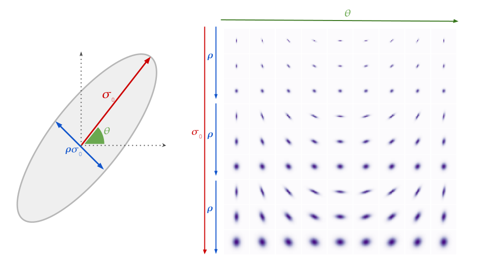 |
| Gaussian blur model and example blur kernels. Each row of the plot on the right represents possible combinations of σ0, ρ and θ. We show three different σ0 values with three different ρ values for each. |
Computing and removing blur without noticeable delay for the user requires an algorithm that is much more computationally efficient than existing approaches, which typically cannot be executed on a mobile device. We rely on an intriguing empirical observation: the maximal value of the image gradient across all directions at any point in a sharp image follows a particular distribution. Finding the maximum gradient value is efficient, and can yield a reliable estimate of the strength of the blur in the given direction. With this information in hand, we can directly recover the parameters that characterize the blur.
Polyblur: Removing Blur by Re-blurring
To recover the sharp image given the estimated blur, we would (in theory) need to solve a numerically unstable inverse problem (i.e., deblurring). The inversion problem grows exponentially more unstable with the strength of the blur. As such, we target the case of mild blur removal. That is, we assume that the image at hand is not so blurry as to be beyond practical repair. This enables a more practical approach — by carefully combining different re-applications of an operator we can approximate its inverse.
 |
 |
| Mild blur, as shown in these examples, can be effectively removed by combining multiple applications of the estimated blur. |
This means, rather counterintuitively, that we can deblur an image by re-blurring it several times with the estimated blur kernel. Each application of the (estimated) blur corresponds to a first order polynomial, and the repeated applications (adding or subtracting) correspond to higher order terms in a polynomial. A key aspect of this approach, which we call polyblur, is that it is very fast, because it only requires a few applications of the blur itself. This allows it to operate on megapixel images in a fraction of a second on a typical mobile device. The degree of the polynomial and its coefficients are set to invert the blur without boosting noise and other unwanted artifacts.
 |
| The deblurred image is generated by adding and subtracting multiple re-applications of the estimated blur (polyblur). |
Integration with Google Photos
The innovations described here have been integrated and made available to users in the Google Photos image editor in two new adjustment sliders called “Denoise” and “Sharpen”. These features allow users to improve the quality of everyday images, from any capture device. The features often complement each other, allowing both denoising to reduce unwanted artifacts, and sharpening to bring clarity to the image subjects. Try using this pair of tools in tandem in your images for best results. To learn more about the details of the work described here, check out our papers on polyblur and pull-push denoising. To see some examples of the effect of our denoising and sharpening up close, have a look at the images in this album.
Acknowledgements
The authors gratefully acknowledge the contributions of Ignacio Garcia-Dorado, Ryan Campbell, Damien Kelly, Peyman Milanfar, and John Isidoro. We are also thankful for support and feedback from Navin Sarma, Zachary Senzer, Brandon Ruffin, and Michael Milne.
1 The original pull-push algorithm was developed as an efficient scattered data interpolation method to estimate and fill in the missing pixels in an image where only a subset of the pixels are specified. Here, we extend its methodology and present a data-dependent multiscale algorithm for denoising images efficiently. ↩
In fall of 2019, we demonstrated that the Sycamore quantum processor could outperform the most powerful classical computers when applied to a tailor-made problem. The next challenge is to extend this result to solve practical problems in materials science, chemistry and physics. But going beyond the capabilities of classical computers for these problems is challenging and will require new insights to achieve state-of-the-art accuracy. Generally, the difficulty in performing quantum simulations of such physical problems is rooted in the wave nature of quantum particles, where deviations in the initial setup, interference from the environment, or small errors in the calculations can lead to large deviations in the computational result.
In two upcoming publications, we outline a blueprint for achieving record levels of precision for the task of simulating quantum materials. In the first work, we consider one-dimensional systems, like thin wires, and demonstrate how to accurately compute electronic properties, such as current and conductance. In the second work, we show how to map the Fermi-Hubbard model, which describes interacting electrons, to a quantum processor in order to simulate important physical properties. These works take a significant step towards realizing our long-term goal of simulating more complex systems with practical applications, like batteries and pharmaceuticals.
 |
| A bottom view of one of the quantum dilution refrigerators during maintenance. During the operation, the microwave wires that are floating in this image are connected to the quantum processor, e.g., the Sycamore chip, bringing the temperature of the lowest stage to a few tens of milli-degrees above absolute zero temperature. |
Computing Electronic Properties of Quantum Materials
In “Accurately computing electronic properties of a quantum ring”, to be published in Nature, we show how to reconstruct key electronic properties of quantum materials. The focus of this work is on one-dimensional conductors, which we simulate by forming a loop out of 18 qubits on the Sycamore processor in order to mimic a very narrow wire. We illustrate the underlying physics through a series of simple text-book experiments, starting with a computation of the “band-structure” of this wire, which describes the relationship between the energy and momentum of electrons in the metal. Understanding such structure is a key step in computing electronic properties such as current and conductance. Despite being an 18-qubit algorithm consisting of over 1,400 logical operations, a significant computational task for near-term devices, we are able to achieve a total error as low as 1%.
The key insight enabling this level of accuracy stems from robust properties of the Fourier transform. The quantum signal that we measure oscillates in time with a small number of frequencies. Taking a Fourier transform of this signal reveals peaks at the oscillation frequencies (in this case, the energy of electrons in the wire). While experimental imperfections affect the height of the observed peaks (corresponding to the strength of the oscillation), the center frequencies are robust to these errors. On the other hand, the center frequencies are especially sensitive to the physical properties of the wire that we hope to study (e.g., revealing small disorders in the local electric field felt by the electrons). The essence of our work is that studying quantum signals in the Fourier domain enables robust protection against experimental errors while providing a sensitive probe of the underlying quantum system.
 |
| (Left) Schematic of the 54-qubit quantum processor, Sycamore. Qubits are shown as gray crosses and tunable couplers as blue squares. Eighteen of the qubits are isolated to form a ring. (Middle) Fourier transform of the measured quantum signal. Peaks in the Fourier spectrum correspond to the energy of electrons in the ring. Each peak can be associated with a traveling wave that has fixed momentum. (Right) The center frequency of each peak (corresponding to the energy of electrons in the wire) is plotted versus the peak index (corresponding to the momentum). The measured relationship between energy and momentum is referred to as the ‘band structure’ of the quantum wire and provides valuable information about electronic properties of the material, such as current and conductance. |
Quantum Simulation of the Fermi-Hubbard Model
In “Observation of separated dynamics of charge and spin in the Fermi-Hubbard model”, we focus on the dynamics of interacting electrons. Interactions between particles give rise to novel phenomena such as high temperature superconductivity and spin-charge separation. The simplest model that captures this behavior is known as the Fermi-Hubbard model. In materials such as metals, the atomic nuclei form a crystalline lattice and electrons hop from lattice site to lattice site carrying electrical current. In order to accurately model these systems, it is necessary to include the repulsion that electrons feel when getting close to one another. The Fermi-Hubbard model captures this physics with two simple parameters that describe the hopping rate (J) and the repulsion strength (U).
We realize the dynamics of this model by mapping the two physical parameters to logical operations on the qubits of the processor. Using these operations, we simulate a state of the electrons where both the electron charge and spin densities are peaked near the center of the qubit array. As the system evolves, the charge and spin densities spread at different rates due to the strong correlations between electrons. Our results provide an intuitive picture of interacting electrons and serve as a benchmark for simulating quantum materials with superconducting qubits.
 |
| (Left top) Illustration of the one-dimensional Fermi-Hubbard model in a periodic potential. Electrons are shown in blue, with their spin indicated by the connected arrow. J, the distance between troughs in the electric potential field, reflects the “hopping” rate, i.e., the rate at which electrons transition from one trough in the potential to another, and U, the amplitude, represents the strength of repulsion between electrons. (Left bottom) The simulation of the model on a qubit ladder, where each qubit (square) represents a fermionic state with spin-up or spin-down (arrows). (Right) Time evolution of the model reveals separated spreading rates of charge and spin. Points and solid lines represent experimental and numerical exact results, respectively. At t = 0, the charge and spin densities are peaked at the middle sites. At later times, the charge density spreads and reaches the boundaries faster than the spin density. |
Conclusion
Quantum processors hold the promise to solve computationally hard tasks beyond the capability of classical approaches. However, in order for these engineered platforms to be considered as serious contenders, they must offer computational accuracy beyond the current state-of-the-art classical methods. In our first experiment, we demonstrate an unprecedented level of accuracy in simulating simple materials, and in our second experiment, we show how to embed realistic models of interacting electrons into a quantum processor. It is our hope that these experimental results help progress the goal of moving beyond the classical computing horizon.
Advances on neural machine translation (NMT) have enabled more natural and fluid translations, but they still can reflect the societal biases and stereotypes of the data they’re trained on. As such, it is an ongoing goal at Google to develop innovative techniques to reduce gender bias in machine translation, in alignment with our AI Principles.
One research area has been using context from surrounding sentences or passages to improve gender accuracy – this is a challenge because traditional NMT methods translate sentences individually, but gendered information is not always explicitly stated in each individual sentence. For example, in the following passage in Spanish (a language where subjects aren’t always explicitly mentioned), the first sentence refers explicitly to Marie Curie as the subject, but the second one doesn’t explicitly mention the subject. In isolation, this second sentence could refer to a person of any gender. When translating to English, however, a pronoun needs to be picked, and the information needed for an accurate translation is in the first sentence.
| Spanish Text | Translation to English |
| Marie Curie nació en Varsovia. Fue la primera persona en recibir dos premios Nobel en distintas especialidades. | Marie Curie was born in Warsaw. She was the first person to receive two Nobel Prizes in different specialties. |
Advancing translation techniques beyond single sentences requires new metrics for measuring progress and new datasets with the most common context-related errors. Adding to this challenge is the fact that translation errors related to gender (such as picking the correct pronoun or having gender agreement) are particularly sensitive because they may directly refer to people and how they self identify.
To help facilitate progress against the common challenges on contextual translation (e.g., pronoun drop, gender agreement and accurate possessives), we are releasing the Translated Wikipedia Biographies dataset, which can be used to evaluate the gender bias of translation models. Our intent with this release is to support long-term improvements on ML systems focused on pronouns and gender in translation by providing a benchmark in which translations’ accuracy can be measured pre- and post-model changes.
A Source of Common Translation Errors
Because they are well-written, geographically diverse, contain multiple sentences, and refer to subjects in the third person (so contain plenty of pronouns), Wikipedia biographies offer a high potential for common translation errors associated with gender. These often occur when articles refer to a person explicitly in early sentences of a paragraph, but there is no explicit mention of the person in later sentences. Some examples:
| Translation Error | Text | Translation | ||
| Pro-drop in Spanish → English | Marie Curie nació en Varsovia. Recibió el Premio Nobel en 1903 y en 1911. | Marie Curie was born in Warsaw. He received the Nobel Prize in 1903 and in 1911. | ||
| Neutral possessives in Spanish → English | Marie Curie nació en Varsovia. Su carrera profesional fue desarrollada en Francia. | Marie Curie was born in Warsaw. His professional career was developed in France. | ||
| Gender agreement in English → German | Marie Curie was born in Warsaw. The distinguished scientist received the Nobel Prize in 1903 and in 1911. | Marie Curie wurde in Varsovia geboren. Der angesehene Wissenschaftler erhielt 1903 und 1911 den Nobelpreis. | ||
| Gender agreement in English → Spanish | Marie Curie was born in Warsaw. The distinguished scientist received the Nobel Prize in 1903 and in 1911. | Marie Curie nació en Varsovia. El distinguido científico recibió el Premio Nobel en 1903 y en 1911. | ||
Building the Dataset
The Translated Wikipedia Biographies dataset has been designed to analyze common gender errors in machine translation such as those illustrated above. Each instance of the dataset represents a person (identified in the biographies as feminine or masculine), a rock band or a sports team (considered genderless). Each instance is represented by a long text translation of 8 to 15 connected sentences referring to that central subject (the person, rock band, or sports team). Articles are written in native English and have been professionally translated to Spanish and German. For Spanish, translations were optimized for pronoun-drop, so the same set could be used to analyze pro-drop (Spanish → English) and gender agreement (English → Spanish).
The dataset was built by selecting a group of instances that has equal representation across geographies and genders. To do this, we extracted biographies from Wikipedia according to occupation, profession, job and/or activity. To ensure an unbiased selection of occupations, we chose 9 occupations that represented a range of stereotypical gender associations (either feminine, masculine, or neither) based on Wikipedia statistics. Then, to mitigate any geography-based bias, we divided all these instances based on geographical diversity. For each occupation category, we looked to have one candidate per region (using regions from census.gov as a proxy of geographical diversity). When an instance was associated with a region, we checked that the selected person had a relevant relationship with a country that belongs to a designated region (nationality, place of birth, lived for a big portion of their life, etc.). By using this criteria, the dataset contains entries about individuals from more than 90 countries and all regions of the world.
Although gender is non-binary, we focused on having equal representation of “feminine” and “masculine” entities. It’s worth mentioning that because the entities are represented as such on Wikipedia, the set doesn’t include individuals that identify as non-binary, as unfortunately there are not enough instances currently represented in Wikipedia to accurately reflect the non-binary community. To label each instance as “feminine” or “masculine” we relied on the biographical information from Wikipedia, which contained gender-specific references to the person (she, he, woman, son, father, etc.).
After applying all these filters, we randomly selected an instance for each occupation-region-gender triplet. For each occupation, there are 2 biographies (one masculine and one feminine), for each of the 7 geographic regions.
Finally, we added 12 instances with no gender. We picked rock bands and sports teams because they are usually referred to by non-gendered third person pronouns (such as “it” or singular “they”). The purpose of including these instances is to study over triggering (i.e., when models learn that they are rewarded for producing gender-specific pronouns, soproduce these pronouns in cases where they shouldn’t).
Results and Applications
This dataset enables a new method of evaluation for gender bias reduction in machine translations (introduced in a previous post). Because each instance refers to a subject with a known gender, we can compute the accuracy of the gender-specific translations that refer to this subject. This computation is easier when translating into English (cases of languages with prodrop or neutral pronouns) since computation is mainly based on gender-specific pronouns in English. In these cases, the gender datasets have allowed us to observe a 67% reduction in errors on context-aware models vs. previous models. As mentioned before, the neutral entities have allowed us to discover cases of over triggering like the usage of feminine or masculine pronouns to refer to genderless entities. This new dataset also enables new research directions into the performance of different models across types of occupations or geographic regions.
As an example, the dataset allowed us to discover the following improvements in an excerpt of the translated biography of Marie Curie from Spanish.
 |
| Translation result with the previous NMT model. |
 |
| Translation result with the new contextual model. |
Conclusion
This Translated Wikipedia Biographies dataset is the result of our own studies and work on identifying biases associated with gender and machine translation. This set focuses on a specific problem related to gender bias and doesn’t aim to cover the whole problem. It’s worth mentioning that by releasing this dataset, we don’t aim to be prescriptive in determining what’s the optimal approach to address gender bias. This contribution aims to foster progress on this challenge across the global research community.
Acknowledgements
The datasets were built with help from Anja Austermann, Melvin Johnson, Michelle Linch, Mengmeng Niu, Mahima Pushkarna, Apu Shah, Romina Stella, and Kellie Webster.
Each person’s genome, which collectively encodes the biochemical machinery they are born with, is composed of over 3 billion letters of DNA. However, only a small subset of the genome (~4-5 million positions) varies between two people. Nonetheless, each person’s unique genome interacts with the environment they experience to determine the majority of their health outcomes. A key method of understanding the relationship between genetic variants and traits is a genome-wide association study (GWAS), in which each genetic variant present in a cohort is individually examined for correlation with the trait of interest. GWAS results can be used to identify and prioritize potential therapeutic targets by identifying genes that are strongly associated with a disease of interest, and can also be used to build a polygenic risk score (PRS) to predict disease predisposition based on the combined influence of variants present in an individual. However, while accurate measurement of traits in an individual (called phenotyping) is essential to GWAS, it often requires painstaking expert curation and/or subjective judgment calls.
In “Large-scale machine learning-based phenotyping significantly improves genomic discovery for optic nerve head morphology”, we demonstrate how using machine learning (ML) models to classify medical imaging data can be used to improve GWAS. We describe how models can be trained for phenotypes to generate trait predictions and how these predictions are used to identify novel genetic associations. We then show that the novel associations discovered improve PRS accuracy and, using glaucoma as an example, that the improvements for anatomical eye traits relate to human disease. We have released the model training code and detailed documentation for its use on our Genomics Research GitHub repository.
Identifying genetic variants associated with eye anatomical traits
Previous work has demonstrated that ML models can identify eye diseases, skin diseases, and abnormal mammogram results with accuracy approaching or exceeding state-of-the-art methods by domain experts. Because identifying disease is a subset of phenotyping, we reasoned that ML models could be broadly used to improve the speed and quality of phenotyping for GWAS.
To test this, we chose a model that uses a fundus image of the eye to accurately predict whether a patient should be referred for assessment for glaucoma. This model uses the fundus images to predict the diameters of the optic disc (the region where the optic nerve connects to the retina) and the optic cup (a whitish region in the center of the optic disc). The ratio of the diameters of these two anatomical features (called the vertical cup-to-disc ratio, or VCDR) correlates strongly with glaucoma risk.
 |
| A representative retinal fundus image showing the vertical cup-to-disc ratio, which is an important diagnostic measurement for glaucoma. |
We applied this model to predict VCDR in all fundus images from individuals in the UK Biobank, which is the world’s largest dataset available to researchers worldwide for health-related research in the public interest, containing extensive phenotyping and genetic data for ~500,000 pseudonymized (the UK Biobank’s standard for de-identification) individuals. We then performed GWAS in this dataset to identify genetic variants that are associated with the model-based predictions of VCDR.
 |
| Applying a VCDR prediction model trained on clinical data to generate predicted values for VCDR to enable discovery of genetic associations for the VCDR trait. |
The ML-based GWAS identified 156 distinct genomic regions associated with VCDR. We compared these results to a VCDR GWAS conducted by another group on the same UK Biobank data, Craig et al. 2020, where experts had painstakingly labeled all images for VCDR. The ML-based GWAS replicates 62 of the 65 associations found in Craig et al., which indicates that the model accurately predicts VCDR in the UK Biobank images. Additionally, the ML-based GWAS discovered 93 novel associations.
 |
| Number of statistically significant GWAS associations discovered by exhaustive expert labeling approach (Craig et al., left), and by our ML-based approach (right), with shared associations in the middle. |
The ML-based GWAS improves polygenic model predictions
To validate that the novel associations discovered in the ML-based GWAS are biologically relevant, we developed independent PRSes using the Craig et al. and ML-based GWAS results, and tested their ability to predict human-expert-labeled VCDR in a subset of UK Biobank as well as a fully independent cohort (EPIC-Norfolk). The PRS developed from the ML-based GWAS showed greater predictive ability than the PRS built from the expert labeling approach in both datasets, providing strong evidence that the novel associations discovered by the ML-based method influence VCDR biology, and suggesting that the improved phenotyping accuracy (i.e., more accurate VCDR measurement) of the model translates into a more powerful GWAS.
 |
| The correlation between a polygenic risk score (PRS) for VCDR generated from the ML-based approach and the exhaustive expert labeling approach (Craig et al.). In these plots, higher values on the y-axis indicate a greater correlation and therefore greater prediction from only the genetic data. [* — p ≤ 0.05; *** — p ≤ 0.001] |
As a second validation, because we know that VCDR is strongly correlated with glaucoma, we also investigated whether the ML-based PRS was correlated with individuals who had either self-reported that they had glaucoma or had medical procedure codes suggestive of glaucoma or glaucoma treatment. We found that the PRS for VCDR determined using our model predictions were also predictive of the probability that an individual had indications of glaucoma. Individuals with a PRS 2.5 or more standard deviations higher than the mean were more than 3 times as likely to have glaucoma in this cohort. We also observed that the VCDR PRS from ML-based phenotypes was more predictive of glaucoma than the VCDR PRS produced from the extensive manual phenotyping.
 |
| The odds ratio of glaucoma (self-report or ICD code) stratified by the PRS for VCDR determined using the ML-based phenotypes (in standard deviations from the mean). In this plot, the y-axis shows the probability that the individual has glaucoma relative to the baseline rate (represented by the dashed line). The x-axis shows standard deviations from the mean for the PRS. Data are visualized as a standard box plot, which illustrates values for the mean (the orange line), first and third quartiles, and minimum and maximum. |
Conclusion
We have shown that ML models can be used to quickly phenotype large cohorts for GWAS, and that these models can increase statistical power in such studies. Although these examples were shown for eye traits predicted from retinal imaging, we look forward to exploring how this concept could generally apply to other diseases and data types.
Acknowledgments
We would like to especially thank co-author Dr. Anthony Khawaja of Moorfields Eye Hospital for contributing his extensive medical expertise. We also recognize the efforts of Professor Jamie Craig and colleagues for their exhaustive labeling of UK Biobank images, which allowed us to make comparisons with our method. Several authors of that work, as well as Professor Stuart MacGregor and collaborators in Australia and at Max Kelsen have independently replicated these findings, and we value these scientific contributions as well.
Quantum computing has rapidly advanced in both theory and practice in recent years, and with it the hope for the potential impact in real applications. One key area of interest is how quantum computers might affect machine learning. We recently demonstrated experimentally that quantum computers are able to naturally solve certain problems with complex correlations between inputs that can be incredibly hard for traditional, or “classical”, computers. This suggests that learning models made on quantum computers may be dramatically more powerful for select applications, potentially boasting faster computation, better generalization on less data, or both. Hence it is of great interest to understand in what situations such a “quantum advantage” might be achieved.
The idea of quantum advantage is typically phrased in terms of computational advantages. That is, given some task with well defined inputs and outputs, can a quantum computer achieve a more accurate result than a classical machine in a comparable runtime? There are a number of algorithms for which quantum computers are suspected to have overwhelming advantages, such as Shor’s factoring algorithm for factoring products of large primes (relevant to RSA encryption) or the quantum simulation of quantum systems. However, the difficulty of solving a problem, and hence the potential advantage for a quantum computer, can be greatly impacted by the availability of data. As such, understanding when a quantum computer can help in a machine learning task depends not only on the task, but also the data available, and a complete understanding of this must include both.
In “Power of data in quantum machine learning”, published in Nature Communications, we dissect the problem of quantum advantage in machine learning to better understand when it will apply. We show how the complexity of a problem formally changes with the availability of data, and how this sometimes has the power to elevate classical learning models to be competitive with quantum algorithms. We then develop a practical method for screening when there may be a quantum advantage for a chosen set of data embeddings in the context of kernel methods. We use the insights from the screening method and learning bounds to introduce a novel method that projects select aspects of feature maps from a quantum computer back into classical space. This enables us to imbue the quantum approach with additional insights from classical machine learning that shows the best empirical separation in quantum learning advantages to date.
Computational Power of Data
The idea of quantum advantage over a classical computer is often framed in terms of computational complexity classes. Examples such as factoring large numbers and simulating quantum systems are classified as bounded quantum polynomial time (BQP) problems, which are those thought to be handled more easily by quantum computers than by classical systems. Problems easily solved on classical computers are called bounded probabilistic polynomial (BPP) problems.
We show that learning algorithms equipped with data from a quantum process, such as a natural process like fusion or chemical reactions, form a new class of problems (which we call BPP/Samp) that can efficiently perform some tasks that traditional algorithms without data cannot, and is a subclass of the problems efficiently solvable with polynomial sized advice (P/poly). This demonstrates that for some machine learning tasks, understanding the quantum advantage requires examination of available data as well.

Geometric Test for Quantum Learning Advantage
Informed by the results that the potential for advantage changes depending on the availability of data, one may ask how a practitioner can quickly evaluate if their problem may be well suited for a quantum computer. To help with this, we developed a workflow for assessing the potential for advantage within a kernel learning framework. We examined a number of tests, the most powerful and informative of which was a novel geometric test we developed.
In quantum machine learning methods, such as quantum neural networks or quantum kernel methods, a quantum program is often divided into two parts, a quantum embedding of the data (an embedding map for the feature space using a quantum computer), and the evaluation of a function applied to the data embedding. In the context of quantum computing, quantum kernel methods make use of traditional kernel methods, but use the quantum computer to evaluate part or all of the kernel on the quantum embedding, which has a different geometry than a classical embedding. It was conjectured that a quantum advantage might arise from the quantum embedding, which might be much better suited to a particular problem than any accessible classical geometry.
We developed a quick and rigorous test that can be used to quickly compare a particular quantum embedding, kernel, and data set to a range of classical kernels and assess if there is any opportunity for quantum advantage across, e.g., possible label functions such as those used for image recognition tasks. We define a geometric constant g, which quantifies the amount of data that could theoretically close that gap, based on the geometric test. This is an extremely useful technique for deciding, based on data constraints, if a quantum solution is right for the given problem.
Projected Quantum Kernel Approach
One insight revealed by the geometric test, was that existing quantum kernels often suffered from a geometry that was easy to best classically because they encouraged memorization, instead of understanding. This inspired us to develop a projected quantum kernel, in which the quantum embedding is projected back to a classical representation. While this representation is still hard to compute with a classical computer directly, it comes with a number of practical advantages in comparison to staying in the quantum space entirely.
 |
| Geometric quantity g, which quantifies the potential for quantum advantage, depicted for several embeddings, including the projected quantum kernel introduced here. |
By selectly projecting back to classical space, we can retain aspects of the quantum geometry that are still hard to simulate classically, but now it is much easier to develop distance functions, and hence kernels, that are better behaved with respect to modest changes in the input than was the original quantum kernel. In addition the projected quantum kernel facilitates better integration with powerful non-linear kernels (like a squared exponential) that have been developed classically, which is much more challenging to do in the native quantum space.
This projected quantum kernel has a number of benefits over previous approaches, including an improved ability to describe non-linear functions of the existing embedding, a reduction in the resources needed to process the kernel from quadratic to linear with the number of data points, and the ability to generalize better at larger sizes. The kernel also helps to expand the geometric g, which helps to ensure the greatest potential for quantum advantage.
Data Sets Exhibit Learning Advantages
The geometric test quantifies potential advantage for all possible label functions, however in practice we are most often interested in specific label functions. Using learning theoretic approaches, we also bound the generalization error for specific tasks, including those which are definitively quantum in origin. As the advantage of a quantum computer relies on its ability to use many qubits simultaneously but previous approaches scale poorly in number of qubits, it is important to verify the tasks at reasonably large qubit sizes ( > 20 ) to ensure a method has the potential to scale to real problems. For our studies we verified up to 30 qubits, which was enabled by the open source tool, TensorFlow-Quantum, enabling scaling to petaflops of compute.
Interestingly, we showed that many naturally quantum problems, even up to 30 qubits, were readily handled by classical learning methods when sufficient data were provided. Hence one conclusion is that even for some problems that look quantum, classical machine learning methods empowered by data can match the power of quantum computers. However, using the geometric construction in combination with the projected quantum kernel, we were able to construct a data set that exhibited an empirical learning advantage for a quantum model over a classical one. Thus, while it remains an open question to find such data sets in natural problems, we were able to show the existence of label functions where this can be the case. Although this problem was engineered and a quantum computational advantage would require the embeddings to be larger and more challenging, this work represents an important step in understanding the role data plays in quantum machine learning.
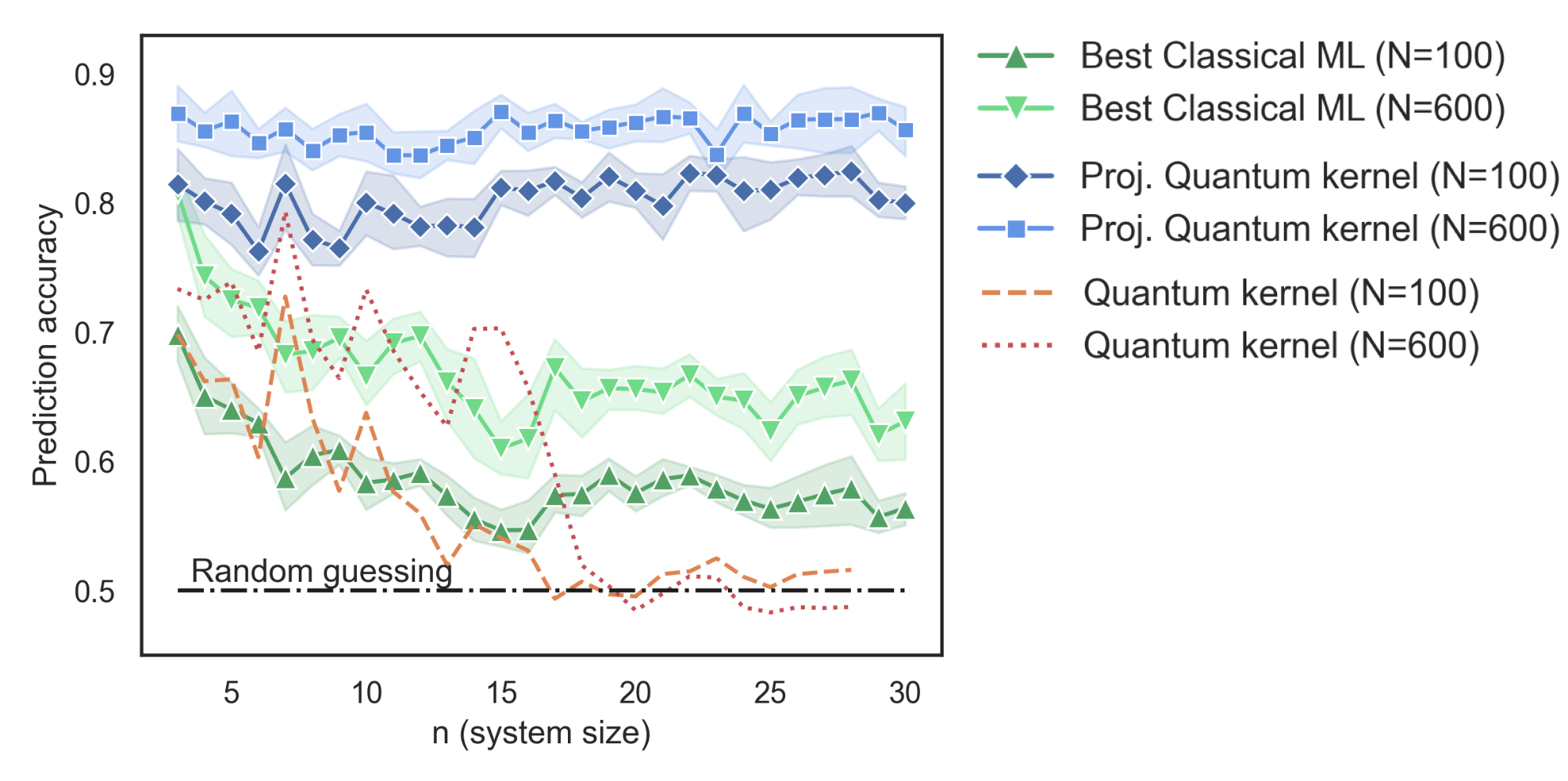 |
| Prediction accuracy as a function of the number of qubits (n) for a problem engineered to maximize the potential for learning advantage in a quantum model. The data is shown for two different sizes of training data (N). |
For this problem, we scaled up the number of qubits (n) and compared the prediction accuracy of the projected quantum kernel to existing kernel approaches and the best classical machine learning model in our dataset. Moreover, a key takeaway from these results is that although we showed the existence of datasets where a quantum computer has an advantage, for many quantum problems, classical learning methods were still the best approach. Understanding how data can affect a given problem is a key factor to consider when discussing quantum advantage in learning problems, unlike traditional computation problems for which that is not a consideration.
Conclusions
When considering the ability of quantum computers to aid in machine learning, we have shown that the availability of data fundamentally changes the question. In our work, we develop a practical set of tools for examining these questions, and use them to develop a new projected quantum kernel method that has a number of advantages over existing approaches. We build towards the largest numerical demonstration to date, 30 qubits, of potential learning advantages for quantum embeddings. While a complete computational advantage on a real world application remains to be seen, this work helps set the foundation for the path forward. We encourage any interested readers to check out both the paper and related TensorFlow-Quantum tutorials that make it easy to build on this work.
Acknowledgements
We would like to acknowledge our co-authors on this paper — Michael Broughton, Masoud Mohseni, Ryan Babbush, Sergio Boixo, and Hartmut Neven, as well as the entirety of the Google Quantum AI team. In addition, we acknowledge valuable help and feedback from Richard Kueng, John Platt, John Preskill, Thomas Vidick, Nathan Wiebe, Chun-Ju Wu, and Balint Pato.
1Current affiliation — Institute for Quantum Information and Matter and Department of Computing and Mathematical Sciences, Caltech, Pasadena, CA, USA↩
Categories
Google at CVPR 2021
This week marks the start of the 2021 Conference on Computer Vision and Pattern Recognition (CVPR 2021), the premier annual computer vision event consisting of the main conference, workshops and tutorials. As a leader in computer vision research and a Champion Level Sponsor, Google will have a strong presence at CVPR 2021, with over 70 publications accepted, along with the organization of and participation in multiple workshops and tutorials.
If you are participating in CVPR this year, please visit our virtual booth to learn about Google research into the next generation of intelligent systems that utilize the latest machine learning techniques applied to various areas of machine perception.
You can also learn more about our research being presented at CVPR 2021 in the list below (Google affiliations in bold).
Organizing Committee Members
General Chair: Rahul Sukthankar
Finance Chair: Ramin Zabih
Workshop Chair: Caroline Pantofaru
Area Chairs: Chen Sun, Golnaz Ghiasi, Jonathan Barron, Kostas Rematas, Negar Rostamzadeh, Noah Snavely, Sanmi Koyejo, Tsung-Yi Lin
Publications
Cross-Modal Contrastive Learning for Text-to-Image Generation (see the blog post)
Han Zhang, Jing Yu Koh, Jason Baldridge, Honglak Lee*, Yinfei Yang
Learning Graph Embeddings for Compositional Zero-Shot Learning
Muhammad Ferjad Naeem, Yongqin Xian, Federico Tombari, Zeynep Akata
SPSG: Self-Supervised Photometric Scene Generation From RGB-D Scans
Angela Dai, Yawar Siddiqui, Justus Thies, Julien Valentin, Matthias Nießner
3D-MAN: 3D Multi-Frame Attention Network for Object Detection
Zetong Yang*, Yin Zhou, Zhifeng Chen, Jiquan Ngiam
MIST: Multiple Instance Spatial Transformer
Baptiste Angles, Yuhe Jin, Simon Kornblith, Andrea Tagliasacchi, Kwang Moo Yi
OCONet: Image Extrapolation by Object Completion
Richard Strong Bowen*, Huiwen Chang, Charles Herrmann*, Piotr Teterwak*, Ce Liu, Ramin Zabih
Ranking Neural Checkpoints
Yandong Li, Xuhui Jia, Ruoxin Sang, Yukun Zhu, Bradley Green, Liqiang Wang, Boqing Gong
LipSync3D: Data-Efficient Learning of Personalized 3D Talking Faces From Video Using Pose and Lighting Normalization
Avisek Lahiri, Vivek Kwatra, Christian Frueh, John Lewis, Chris Bregler
Differentiable Patch Selection for Image Recognition
Jean-Baptiste Cordonnier*, Aravindh Mahendran, Alexey Dosovitskiy, Dirk Weissenborn, Jakob Uszkoreit, Thomas Unterthiner
HumanGPS: Geodesic PreServing Feature for Dense Human Correspondences
Feitong Tan, Danhang Tang, Mingsong Dou, Kaiwen Guo, Rohit Pandey, Cem Keskin, Ruofei Du, Deqing Sun, Sofien Bouaziz, Sean Fanello, Ping Tan, Yinda Zhang
VIP-DeepLab: Learning Visual Perception With Depth-Aware Video Panoptic Segmentation (see the blog post)
Siyuan Qiao*, Yukun Zhu, Hartwig Adam, Alan Yuille, Liang-Chieh Chen
DeFMO: Deblurring and Shape Recovery of Fast Moving Objects
Denys Rozumnyi, Martin R. Oswald, Vittorio Ferrari, Jiri Matas, Marc Pollefeys
HDMapGen: A Hierarchical Graph Generative Model of High Definition Maps
Lu Mi, Hang Zhao, Charlie Nash, Xiaohan Jin, Jiyang Gao, Chen Sun, Cordelia Schmid, Nir Shavit, Yuning Chai, Dragomir Anguelov
Wide-Baseline Relative Camera Pose Estimation With Directional Learning
Kefan Chen, Noah Snavely, Ameesh Makadia
MobileDets: Searching for Object Detection Architectures for Mobile Accelerators
Yunyang Xiong, Hanxiao Liu, Suyog Gupta, Berkin Akin, Gabriel Bender, Yongzhe Wang, Pieter-Jan Kindermans, Mingxing Tan, Vikas Singh, Bo Chen
SMURF: Self-Teaching Multi-Frame Unsupervised RAFT With Full-Image Warping
Austin Stone, Daniel Maurer, Alper Ayvaci, Anelia Angelova, Rico Jonschkowski
Conceptual 12M: Pushing Web-Scale Image-Text Pre-Training To Recognize Long-Tail Visual Concepts
Soravit Changpinyo, Piyush Sharma, Nan Ding, Radu Soricut
Uncalibrated Neural Inverse Rendering for Photometric Stereo of General Surfaces
Berk Kaya, Suryansh Kumar, Carlos Oliveira, Vittorio Ferrari, Luc Van Gool
MeanShift++: Extremely Fast Mode-Seeking With Applications to Segmentation and Object Tracking
Jennifer Jang, Heinrich Jiang
Repopulating Street Scenes
Yifan Wang*, Andrew Liu, Richard Tucker, Jiajun Wu, Brian L. Curless, Steven M. Seitz, Noah Snavely
MaX-DeepLab: End-to-End Panoptic Segmentation With Mask Transformers (see the blog post)
Huiyu Wang*, Yukun Zhu, Hartwig Adam, Alan Yuille, Liang-Chieh Chen
IBRNet: Learning Multi-View Image-Based Rendering
Qianqian Wang, Zhicheng Wang, Kyle Genova, Pratul Srinivasan, Howard Zhou, Jonathan T. Barron, Ricardo Martin-Brualla, Noah Snavely, Thomas Funkhouser
From Points to Multi-Object 3D Reconstruction
Francis Engelmann*, Konstantinos Rematas, Bastian Leibe, Vittorio Ferrari
Learning Compositional Representation for 4D Captures With Neural ODE
Boyan Jiang, Yinda Zhang, Xingkui Wei, Xiangyang Xue, Yanwei Fu
Guided Integrated Gradients: An Adaptive Path Method for Removing Noise
Andrei Kapishnikov, Subhashini Venugopalan, Besim Avci, Ben Wedin, Michael Terry, Tolga Bolukbasi
De-Rendering the World’s Revolutionary Artefacts
Shangzhe Wu*, Ameesh Makadia, Jiajun Wu, Noah Snavely, Richard Tucker, Angjoo Kanazawa
Spatiotemporal Contrastive Video Representation Learning
Rui Qian, Tianjian Meng, Boqing Gong, Ming-Hsuan Yang, Huisheng Wang, Serge Belongie, Yin Cui
Decoupled Dynamic Filter Networks
Jingkai Zhou, Varun Jampani, Zhixiong Pi, Qiong Liu, Ming-Hsuan Yang
NeuralHumanFVV: Real-Time Neural Volumetric Human Performance Rendering Using RGB Cameras
Xin Suo, Yuheng Jiang, Pei Lin, Yingliang Zhang, Kaiwen Guo, Minye Wu, Lan Xu
Regularizing Generative Adversarial Networks Under Limited Data
Hung-Yu Tseng*, Lu Jiang, Ce Liu, Ming-Hsuan Yang, Weilong Yang
SceneGraphFusion: Incremental 3D Scene Graph Prediction From RGB-D Sequences
Shun-Cheng Wu, Johanna Wald, Keisuke Tateno, Nassir Navab, Federico Tombari
NeRV: Neural Reflectance and Visibility Fields for Relighting and View Synthesis
Pratul P. Srinivasan, Boyang Deng, Xiuming Zhang, Matthew Tancik, Ben Mildenhall, Jonathan T. Barron
Adversarially Adaptive Normalization for Single Domain Generalization
Xinjie Fan*, Qifei Wang, Junjie Ke, Feng Yang, Boqing Gong, Mingyuan Zhou
Adaptive Prototype Learning and Allocation for Few-Shot Segmentation
Gen Li, Varun Jampani, Laura Sevilla-Lara, Deqing Sun, Jonghyun Kim, Joongkyu Kim
Adversarial Robustness Across Representation Spaces
Pranjal Awasthi, George Yu, Chun-Sung Ferng, Andrew Tomkins, Da-Cheng Juan
Background Splitting: Finding Rare Classes in a Sea of Background
Ravi Teja Mullapudi, Fait Poms, William R. Mark, Deva Ramanan, Kayvon Fatahalian
Searching for Fast Model Families on Datacenter Accelerators
Sheng Li, Mingxing Tan, Ruoming Pang, Andrew Li, Liqun Cheng, Quoc Le, Norman P. Jouppi
Objectron: A Large Scale Dataset of Object-Centric Videos in the Wild With Pose Annotations (see the blog post)
Adel Ahmadyan, Liangkai Zhang, Jianing Wei, Artsiom Ablavatski, Matthias Grundmann
CutPaste: Self-Supervised Learning for Anomaly Detection and Localization
Chun-Liang Li, Kihyuk Sohn, Jinsung Yoon, Tomas Pfister
Nutrition5k: Towards Automatic Nutritional Understanding of Generic Food
Quin Thames, Arjun Karpur, Wade Norris, Fangting Xia, Liviu Panait, Tobias Weyand, Jack Sim
CReST: A Class-Rebalancing Self-Training Framework for Imbalanced Semi-Supervised Learning
Chen Wei*, Kihyuk Sohn, Clayton Mellina, Alan Yuille, Fan Yang
DetectoRS: Detecting Objects With Recursive Feature Pyramid and Switchable Atrous Convolution
Siyuan Qiao, Liang-Chieh Chen, Alan Yuille
DeRF: Decomposed Radiance Fields
Daniel Rebain, Wei Jiang, Soroosh Yazdani, Ke Li, Kwang Moo Yi, Andrea Tagliasacchi
Variational Transformer Networks for Layout Generation (see the blog post)
Diego Martin Arroyo, Janis Postels, Federico Tombari
Rich Features for Perceptual Quality Assessment of UGC Videos
Yilin Wang, Junjie Ke, Hossein Talebi, Joong Gon Yim, Neil Birkbeck, Balu Adsumilli, Peyman Milanfar, Feng Yang
Complete & Label: A Domain Adaptation Approach to Semantic Segmentation of LiDAR Point Clouds
Li Yi, Boqing Gong, Thomas Funkhouser
Neural Descent for Visual 3D Human Pose and Shape
Andrei Zanfir, Eduard Gabriel Bazavan, Mihai Zanfir, William T. Freeman, Rahul Sukthankar, Cristian Sminchisescu
GDR-Net: Geometry-Guided Direct Regression Network for Monocular 6D Object Pose Estimation
Gu Wang, Fabian Manhardt, Federico Tombari, Xiangyang Ji
Look Before You Speak: Visually Contextualized Utterances
Paul Hongsuck Seo, Arsha Nagrani, Cordelia Schmid
LASR: Learning Articulated Shape Reconstruction From a Monocular Video
Gengshan Yang*, Deqing Sun, Varun Jampani, Daniel Vlasic, Forrester Cole, Huiwen Chang, Deva Ramanan, William T. Freeman, Ce Liu
MoViNets: Mobile Video Networks for Efficient Video Recognition
Dan Kondratyuk, Liangzhe Yuan, Yandong Li, Li Zhang, Mingxing Tan, Matthew Brown, Boqing Gong
No Shadow Left Behind: Removing Objects and Their Shadows Using Approximate Lighting and Geometry
Edward Zhang, Ricardo Martin-Brualla, Janne Kontkanen, Brian Curless
On Robustness and Transferability of Convolutional Neural Networks
Josip Djolonga, Jessica Yung, Michael Tschannen, Rob Romijnders, Lucas Beyer, Alexander Kolesnikov, Joan Puigcerver, Matthias Minderer, Alexander D’Amour, Dan Moldovan, Sylvain Gelly, Neil Houlsby, Xiaohua Zhai, Mario Lucic
Robust and Accurate Object Detection via Adversarial Learning
Xiangning Chen, Cihang Xie, Mingxing Tan, Li Zhang, Cho-Jui Hsieh, Boqing Gong
To the Point: Efficient 3D Object Detection in the Range Image With Graph Convolution Kernels
Yuning Chai, Pei Sun, Jiquan Ngiam, Weiyue Wang, Benjamin Caine, Vijay Vasudevan, Xiao Zhang, Dragomir Anguelov
Bottleneck Transformers for Visual Recognition
Aravind Srinivas, Tsung-Yi Lin, Niki Parmar, Jonathon Shlens, Pieter Abbeel, Ashish Vaswani
Faster Meta Update Strategy for Noise-Robust Deep Learning
Youjiang Xu, Linchao Zhu, Lu Jiang, Yi Yang
Correlated Input-Dependent Label Noise in Large-Scale Image Classification
Mark Collier, Basil Mustafa, Efi Kokiopoulou, Rodolphe Jenatton, Jesse Berent
Learned Initializations for Optimizing Coordinate-Based Neural Representations
Matthew Tancik, Ben Mildenhall, Terrance Wang, Divi Schmidt, Pratul P. Srinivasan, Jonathan T. Barron, Ren Ng
Simple Copy-Paste Is a Strong Data Augmentation Method for Instance Segmentation
Golnaz Ghiasi, Yin Cui, Aravind Srinivas*, Rui Qian, Tsung-Yi Lin, Ekin D. Cubuk, Quoc V. Le, Barret Zoph
Function4D: Real-Time Human Volumetric Capture From Very Sparse Consumer RGBD Sensors
Tao Yu, Zerong Zheng, Kaiwen Guo, Pengpeng Liu, Qionghai Dai, Yebin Liu
RSN: Range Sparse Net for Efficient, Accurate LiDAR 3D Object Detection
Pei Sun, Weiyue Wang, Yuning Chai, Gamaleldin Elsayed, Alex Bewley, Xiao Zhang, Cristian Sminchisescu, Dragomir Anguelov
NeRF in the Wild: Neural Radiance Fields for Unconstrained Photo Collections
Ricardo Martin-Brualla, Noha Radwan, Mehdi S. M. Sajjadi, Jonathan T. Barron, Alexey Dosovitskiy, Daniel Duckworth
Robust Neural Routing Through Space Partitions for Camera Relocalization in Dynamic Indoor Environments
Siyan Dong, Qingnan Fan, He Wang, Ji Shi, Li Yi, Thomas Funkhouser, Baoquan Chen, Leonidas Guibas
Taskology: Utilizing Task Relations at Scale
Yao Lu, Sören Pirk, Jan Dlabal, Anthony Brohan, Ankita Pasad*, Zhao Chen, Vincent Casser, Anelia Angelova, Ariel Gordon
Omnimatte: Associating Objects and Their Effects in Video
Erika Lu, Forrester Cole, Tali Dekel, Andrew Zisserman, William T. Freeman, Michael Rubinstein
AutoFlow: Learning a Better Training Set for Optical Flow
Deqing Sun, Daniel Vlasic, Charles Herrmann, Varun Jampani, Michael Krainin, Huiwen Chang, Ramin Zabih, William T. Freeman, and Ce Liu
Unsupervised Multi-Source Domain Adaptation Without Access to Source Data
Sk Miraj Ahmed, Dripta S. Raychaudhuri, Sujoy Paul, Samet Oymak, Amit K. Roy-Chowdhury
Meta Pseudo Labels
Hieu Pham, Zihang Dai, Qizhe Xie, Minh-Thang Luong, Quoc V. Le
Spatially-Varying Outdoor Lighting Estimation From Intrinsics
Yongjie Zhu, Yinda Zhang, Si Li, Boxin Shi
Learning View-Disentangled Human Pose Representation by Contrastive Cross-View Mutual Information Maximization
Long Zhao*, Yuxiao Wang, Jiaping Zhao, Liangzhe Yuan, Jennifer J. Sun, Florian Schroff, Hartwig Adam, Xi Peng, Dimitris Metaxas, Ting Liu
Benchmarking Representation Learning for Natural World Image Collections
Grant Van Horn, Elijah Cole, Sara Beery, Kimberly Wilber, Serge Belongie, Oisin Mac Aodha
Scaling Local Self-Attention for Parameter Efficient Visual Backbones
Ashish Vaswani, Prajit Ramachandran, Aravind Srinivas, Niki Parmar, Blake Hechtman, Jonathon Shlens
KeypointDeformer: Unsupervised 3D Keypoint Discovery for Shape Control
Tomas Jakab*, Richard Tucker, Ameesh Makadia, Jiajun Wu, Noah Snavely, Angjoo Kanazawa
HITNet: Hierarchical Iterative Tile Refinement Network for Real-time Stereo Matching
Vladimir Tankovich, Christian Häne, Yinda Zhang, Adarsh Kowdle, Sean Fanello, Sofien Bouaziz
POSEFusion: Pose-Guided Selective Fusion for Single-View Human Volumetric Capture
Zhe Li, Tao Yu, Zerong Zheng, Kaiwen Guo, Yebin Liu
Workshops (only Google affiliations are noted)
Media Forensics
Organizers: Christoph Bregler
Safe Artificial Intelligence for Automated Driving
Invited Speakers: Been Kim
VizWiz Grand Challenge
Organizers: Meredith Morris
3D Vision and Robotics
Invited Speaker: Andy Zeng
New Trends in Image Restoration and Enhancement Workshop and Challenges on Image and Video Processing
Organizers: Ming-Hsuan Yang Program Committee: George Toderici, Ming-Hsuan Yang
2nd Workshop on Extreme Vision Modeling
Invited Speakers: Quoc Le, Chen Sun
First International Workshop on Affective Understanding in Video
Organizers: Gautam Prasad, Ting Liu
Adversarial Machine Learning in Real-World Computer Vision Systems and Online Challenges
Program Committee: Nicholas Carlini, Nicolas Papernot
Ethical Considerations in Creative Applications of Computer Vision
Invited Speaker: Alex Hanna Organizers: Negar Rostamzadeh, Emily Denton, Linda Petrini
Visual Question Answering Workshop
Invited Speaker: Vittorio Ferrari
Sixth International Skin Imaging Collaboration (ISIC) Workshop on Skin Image Analysis
Invited Speakers: Sandra Avila Organizers: Yuan Liu Steering Committee: Yuan Liu, Dale Webster
The 4th Workshop and Prize Challenge: Bridging the Gap between Computational Photography and Visual Recognition (UG2+) in Conjunction with IEEE CVPR 2021
Invited Speakers: Peyman Milanfar, Chelsea Finn
The 3rd CVPR Workshop on 3D Scene Understanding for Vision, Graphics, and Robotics
Invited Speaker: Andrea Tagliasacchi
Robust Video Scene Understanding: Tracking and Video Segmentation
Organizers: Jordi Pont-Tuset, Sergi Caelles, Jack Valmadre, Alex Bewley
4th Workshop and Challenge on Learned Image Compression
Invited Speaker: Rianne van den Berg Organizers: George Toderici, Lucas Theis, Johannes Ballé, Eirikur Agustsson, Nick Johnston, Fabian Mentzer
The Third Workshop on Precognition: Seeing Through the Future
Invited Speaker: Anelia Angelova
Organizers: Utsav Prabhu Program Committee: Chen Sun, David Ross
Computational Cameras and Displays
Organizers: Tali Dekel Keynote Talks: Paul Debevec Program Committee: Ayan Chakrabarti, Tali Dekel
2nd Embodied AI Workshop
Organizing Committee: Anthony Francis Challenge Organizers: Peter Anderson, Anthony Francis, Alex Ku, Alexander Toshev Scientific Advisory Board: Alexander Toshev
Responsible Computer Vision
Program Committee: Caroline Pantofaru, Utsav Prabhu, Susanna Ricco, Negar Rostamzadeh, Candice Schumann
Dynamic Neural Networks Meets Computer Vision
Invited Speaker: Azalia Mirhoseini
Interactive Workshop on Bridging the Gap between Subjective and Computational Measurements of Machine Creativity
Invited Speaker: David Bau
GAZE 2021: The 3rd International Workshop on Gaze Estimation and Prediction in the Wild
Organizer: Thabo Beeler Program Committee: Thabo Beeler
Sight and Sound
Organizers: William Freeman
Future of Computer Vision Datasets
Invited Speaker: Emily Denton, Caroline Pantofaru
Open World Vision
Invited Speakers: Rahul Sukthankar
The 3rd Workshop on Learning from Unlabeled Videos
Organizers: Anelia Angelova, Honglak Lee Program Committee: AJ Piergiovanni
4th International Workshop on Visual Odometry and Computer Vision Applications Based on Location Clues — With a Focus on Mobile Platform Applications
Organizers: Anelia Angelova
4th Workshop on Efficient Deep Learning for Computer Vision
Invited Speaker: Andrew Howard
Organizers: Pete Warden, Andrew Howard
Second International Workshop on Large Scale Holistic Video Understanding
Invited Speaker: Cordelia Schmid Program Committee: AJ Piergiovanni Organizers: David Ross
Neural Architecture Search 1st Lightweight NAS Challenge and Moving Beyond
Invited Speakers: Sara Sabour
The Second Workshop on Fair, Data-Efficient, and Trusted Computer Vision
Invited Speakers: Gaurav Aggarwal
The 17th Embedded Vision Workshop
General Chair: Anelia Angelova
8th Workshop on Fine-Grained Visual Categorization
Organizers: Christine Kaeser-Chen, Kimberly Wilber
AI for Content Creation
Invited Speaker: Tali Dekel, Jon Barron, Emily Denton Organizers: Deqing Sun
Frontiers of Monocular 3D Perception
Invited Speakers: Anelia Angelova, Cordelia Schmid, Noah Snavely
Beyond Fairness: Towards a Just, Equitable, and Accountable Computer Vision
Organizers: Emily Denton
The 1st Workshop on Future Video Conferencing
Invited Speakers: Chuo-Ling Chang, Sergi Caelles
Tutorials (only Google affiliations are noted)
Tutorial on Fairness Accountability Transparency and Ethics in Computer Vision
Organizer: Emily Denton
Data-Efficient Learning in An Imperfect World
Organizers: Boqing Gong, Ting Chen
Semantic Segmentation of Point Clouds: a Deep Learning Framework for Cultural Heritage
Invited Speaker: Manzil Zaheer
From VQA to VLN: Recent Advances in Vision-and-Language Research
Organizer: Peter Anderson * Indicates work done while at Google
Categories
Que haja luz: More light for torch!
Today, we’re introducing luz, a high-level interface to torch that lets you train neural networks in a concise, declarative style. In some sense, it is to torch what Keras is to TensorFlow: It provides both a streamlined workflow and powerful ways for customization.