Category: Offsites
Stuff I find valuable at key websites
It might seem reasonable to assume that people’s facial expressions are universal — so, for example, whether a person is from Brazil, India or Canada, their smile upon seeing close friends or their expression of awe at a fireworks display would look essentially the same. But is that really true? Is the association between these facial expressions and their relevant context across geographies indeed universal? What can similarities — or differences — between the situations where someone grins or frowns tell us about how people may be connected across different cultures?
Scientists seeking to answer these questions and to uncover the extent to which people are connected across cultures and geography often use survey-based studies that can rely heavily on local language, norms, and values. However, such studies are not scalable, and often end up with small sample sizes and inconsistent findings.
In contrast to survey-based studies, studying patterns of facial movement provides a more direct understanding of expressive behavior. But analyzing how facial expressions are actually used in everyday life would require researchers to go through millions of hours of real-world footage, which is too time-consuming to do manually. In addition, facial expressions and the contexts in which they are exhibited are complicated, requiring large sample sizes in order to make statistically sound conclusions. While existing studies have produced diverging answers to the question of the universality of facial expressions in given contexts, applying machine learning (ML) in order to appropriately scale the research has the potential to provide clarity.
In “Sixteen facial expressions occur in similar contexts worldwide”, published in Nature, we present research undertaken in collaboration with UC Berkeley to conduct the first large-scale worldwide analysis of how facial expressions are actually used in everyday life, leveraging deep neural networks (DNNs) to drastically scale up expression analysis in a responsible and thoughtful way. Using a dataset of six million publicly available videos across 144 countries, we analyze the contexts in which people use a variety of facial expressions and demonstrate that rich nuances in facial behavior — including subtle expressions — are used in similar social situations around the world.
A Deep Neural Network Measuring Facial Expression
Facial expressions are not static. If one were to examine a person’s expression instant by instant, what might at first appear to be “anger”, may instead end up being “awe”, “surprise” or “confusion”. The interpretation depends on the dynamics of a person’s face as their expression presents itself. The challenge in building a neural network to understand facial expressions, then, is that it must interpret the expression within its temporal context. Training such a system requires a large and diverse, cross-cultural dataset of videos with fully annotated expressions.
To build the dataset, skilled raters manually searched through a broad collection of publicly available videos to identify those likely to contain clips covering all of our pre-selected expression categories. To ensure that the videos matched the region they were assumed to represent, preference in video selection was given to those that included the geographic location of origin. The faces in the videos were then found using a deep convolutional neural network (CNN) — similar to the Google Cloud Face Detection API — that follows faces over the course of the clip using a method based on traditional optical flow. Using an interface similar to Google Crowdsource, annotators then labeled facial expressions across 28 distinct categories if present at any point during the clip. Because the goal was to sample how an average person would perceive an expression, the annotators were not coached or trained, nor were they provided examples or definitions of the target expressions. We discuss additional experiments to evaluate whether the model trained from these annotations was biased below.
 |
| Raters were presented videos with a single face highlighted for their attention. They observed the subject throughout the duration of the clip and annotated the facial expressions they exhibited. (source video) |
The face detection algorithm established a sequence of locations of each face throughout the video. We then used a pre-trained Inception network to extract features representing the most salient aspects of facial expressions from the faces. The features were then fed into a long short-term memory (LSTM) network, a type of recurrent neural network that is able to model how a facial expression might evolve over time due to its ability to remember salient information from the past.
In order to ensure that the model was making consistent predictions across a range of demographic groups, we evaluated the model fairness on an existing dataset that was constructed using similar facial expression labels, targeting a subset of 16 expressions on which it exhibited the best performance.
The model’s performance was consistent across all of the demographic groups represented in the evaluation dataset, which provides supporting evidence that the model trained to annotated facial expressions is not measurably biased. The model’s annotations of those 16 facial expressions across 1,500 images can be explored here.
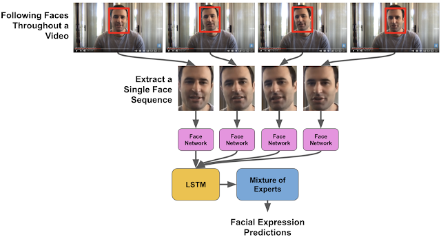 |
| We modeled the selected face in each video by using a CNN to extract features from the face at each frame, which were then fed into an LSTM network to model the changes in the expression over time. (source video) |
Measuring the Contexts Captured in Videos
To understand the context of facial expressions across millions of videos, we used DNNs that could capture the fine-grained content and automatically recognize the context. The first DNN modeled a combination of text features (title and description) associated with a video along with the actual visual content (video-topic model). In addition, we used a DNN that only relied on text features without any visual information (text-topic model). These models predict thousands of labels describing the videos. In our experiments these models were able to identify hundreds of unique contexts (e.g., wedding, sporting event, or fireworks) showcasing the diversity of the data we used for the analysis.
The Covariation Between Expressions and Contexts Around the World
In our first experiment, we analyzed 3 million public videos captured on mobile phones. We chose to focus on mobile uploads because they are more likely to contain natural expressions. We correlated the facial expressions that occurred in the videos to the context annotations derived from the video-topic model. We found 16 kinds of facial expressions had distinct associations with everyday social contexts that were consistent across the world. For instance, the expressions that people associate with amusement occurred more often in videos with practical jokes; expressions that people associate with awe, in videos with fireworks; and triumph, with sporting events. These results have strong implications for discussions about the relative importance of psychologically relevant context in facial expression, compared to other factors, such as those unique to an individual, culture, or society.
Our second experiment analyzed a separate set of 3 million videos, but this time we annotated the contexts with the text-topic model. The results verified that the findings in the first experiment were not driven by subtle influences of facial expressions in the video on the annotations of the video-topic model. In other words we used this experiment to verify our conclusions from the first experiment given the possibility that the video-topic model could implicitly be factoring in facial expressions when computing its content labels.
In both experiments, the correlations between expressions and contexts appeared to be well-preserved across cultures. To quantify exactly how similar the associations between expressions and contexts were across the 12 different world regions we studied, we computed second-order correlations between each pair of regions. These correlations identify the relationships between different expressions and contexts in each region and then compare them with other regions. We found that 70% of the context–expression associations found in each region are shared across the modern world.
Finally, we asked how many of the 16 kinds of facial expression we measured had distinct associations with different contexts that were preserved around the world. To do so, we applied a method called canonical correlations analysis, which showed that all 16 facial expressions had distinct associations that were preserved across the world.
Conclusions
We were able to examine the contexts in which facial expressions occur in everyday life across cultures at an unprecedented scale. Machine learning allowed us to analyze millions of videos across the world and discover evidence supporting hypotheses that facial expressions are preserved to a degree in similar contexts across cultures.
Our results also leave room for cultural differences. Although the correlations between facial expressions and contexts were 70% consistent around the world, they were up to 30% variable across regions. Neighboring world regions generally had more similar associations between facial expressions and contexts than distant world regions, indicating that the geographic spread of human culture may also play a role in the meanings of facial expressions.
This work shows that we can use machine learning to better understand ourselves and identify common communication elements across cultures. Tools such as DNNs give us the opportunity to provide vast amounts of diverse data in service of scientific discovery, enabling more confidence in the statistical conclusions. We hope our work provides a template for using the tools of machine learning in a responsible way and sparks more innovative research in other scientific domains.
Acknowledgements
Special thanks to our co-authors Dacher Keltner from UC Berkeley, along with Florian Schroff, Brendan Jou, and Hartwig Adam from Google Research. We are also grateful for additional support at Google provided by Laura Rapin, Reena Jana, Will Carter, Unni Nair, Christine Robson, Jen Gennai, Sourish Chaudhuri, Greg Corrado, Brian Eoff, Andrew Smart, Raine Serrano, Blaise Aguera y Arcas, Jay Yagnik, and Carson Mcneil.
Large pre-trained natural language processing (NLP) models, such as BERT, RoBERTa, GPT-3, T5 and REALM, leverage natural language corpora that are derived from the Web and fine-tuned on task specific data, and have made significant advances in various NLP tasks. However, natural language text alone represents a limited coverage of knowledge, and facts may be contained in wordy sentences in many different ways. Furthermore, existence of non-factual information and toxic content in text can eventually cause biases in the resulting models.
Alternate sources of information are knowledge graphs (KGs), which consist of structured data. KGs are factual in nature because the information is usually extracted from more trusted sources, and post-processing filters and human editors ensure inappropriate and incorrect content are removed. Therefore, models that can incorporate them carry the advantages of improved factual accuracy and reduced toxicity. However, their different structural format makes it difficult to integrate them with the existing pre-training corpora in language models.
In “Knowledge Graph Based Synthetic Corpus Generation for Knowledge-Enhanced Language Model Pre-training” (KELM), accepted at NAACL 2021, we explore converting KGs to synthetic natural language sentences to augment existing pre-training corpora, enabling their integration into the pre-training of language models without architectural changes. To that end, we leverage the publicly available English Wikidata KG and convert it into natural language text in order to create a synthetic corpus. We then augment REALM, a retrieval-based language model, with the synthetic corpus as a method of integrating natural language corpora and KGs in pre-training. We have released this corpus publicly for the broader research community.
Converting KG to Natural Language Text
KGs consist of factual information represented explicitly in a structured format, generally in the form of [subject entity, relation, object entity] triples, e.g., [10×10 photobooks, inception, 2012]. A group of related triples is called an entity subgraph. An example of an entity subgraph that builds on the previous example of a triple is { [10×10 photobooks, instance of, Nonprofit Organization], [10×10 photobooks, inception, 2012] }, which is illustrated in the figure below. A KG can be viewed as interconnected entity subgraphs.
Converting subgraphs into natural language text is a standard task in NLP known as data-to-text generation. Although there have been significant advances on data-to-text-generation on benchmark datasets such as WebNLG, converting an entire KG into natural text has additional challenges. The entities and relations in large KGs are more vast and diverse than small benchmark datasets. Moreover, benchmark datasets consist of predefined subgraphs that can form fluent meaningful sentences. With an entire KG, such a segmentation into entity subgraphs needs to be created as well.
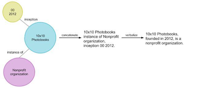 |
| An example illustration of how the pipeline converts an entity subgraph (in bubbles) into synthetic natural sentences (far right). |
In order to convert the Wikidata KG into synthetic natural sentences, we developed a verbalization pipeline named “Text from KG Generator” (TEKGEN), which is made up of the following components: a large training corpus of heuristically aligned Wikipedia text and Wikidata KG triples, a text-to-text generator (T5) to convert the KG triples to text, an entity subgraph creator for generating groups of triples to be verbalized together, and finally, a post-processing filter to remove low quality outputs. The result is a corpus containing the entire Wikidata KG as natural text, which we call the Knowledge-Enhanced Language Model (KELM) corpus. It consists of ~18M sentences spanning ~45M triples and ~1500 relations.
 |
| Converting a KG to natural language, which is then used for language model augmentation |
Integrating Knowledge Graph and Natural Text for Language Model Pre-training
Our evaluation shows that KG verbalization is an effective method of integrating KGs with natural language text. We demonstrate this by augmenting the retrieval corpus of REALM, which includes only Wikipedia text.
To assess the effectiveness of verbalization, we augment the REALM retrieval corpus with the KELM corpus (i.e., “verbalized triples”) and compare its performance against augmentation with concatenated triples without verbalization. We measure the accuracy with each data augmentation technique on two popular open-domain question answering datasets: Natural Questions and Web Questions.
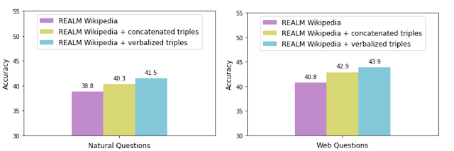 |
Augmenting REALM with even the concatenated triples improves accuracy, potentially adding information not expressed in text explicitly or at all. However, augmentation with verbalized triples allows for a smoother integration of the KG with the natural language text corpus, as demonstrated by the higher accuracy. We also observed the same trend on a knowledge probe called LAMA that queries the model using fill-in-the-blank questions.
Conclusion
With KELM, we provide a publicly-available corpus of a KG as natural text. We show that KG verbalization can be used to integrate KGs with natural text corpora to overcome their structural differences. This has real-world applications for knowledge-intensive tasks, such as question answering, where providing factual knowledge is essential. Moreover, such corpora can be applied in pre-training of large language models, and can potentially reduce toxicity and improve factuality. We hope that this work encourages further advances in integrating structured knowledge sources into pre-training of large language models.
Acknowledgements
This work has been a collaborative effort involving Oshin Agarwal, Heming Ge, Siamak Shakeri and Rami Al-Rfou. We thank William Woods, Jonni Kanerva, Tania Rojas-Esponda, Jianmo Ni, Aaron Cohen and Itai Rolnick for rating a sample of the synthetic corpus to evaluate its quality. We also thank Kelvin Guu for his valuable feedback on the paper.
For the 285 million people around the world living with blindness or low vision, exercising independently can be challenging. Earlier this year, we announced Project Guideline, an early-stage research project, developed in partnership with Guiding Eyes for the Blind, that uses machine learning to guide runners through a variety of environments that have been marked with a painted line. Using only a phone running Guideline technology and a pair of headphones, Guiding Eyes for the Blind CEO Thomas Panek was able to run independently for the first time in decades and complete an unassisted 5K in New York City’s Central Park.
Safely and reliably guiding a blind runner in unpredictable environments requires addressing a number of challenges. Here, we will walk through the technology behind Guideline and the process by which we were able to create an on-device machine learning model that could guide Thomas on an independent outdoor run. The project is still very much under development, but we’re hopeful it can help explore how on-device technology delivered by a mobile phone can provide reliable, enhanced mobility and orientation experiences for those who are blind or low vision.
 |
| Thomas Panek using Guideline technology to run independently outdoors. |
Project Guideline
The Guideline system consists of a mobile device worn around the user’s waist with a custom belt and harness, a guideline on the running path marked with paint or tape, and bone conduction headphones. Core to the Guideline technology is an on-device segmentation model that takes frames from a mobile device’s camera as input and classifies every pixel in the frame into two classes, “guideline” and “not guideline”. This simple confidence mask, applied to every frame, allows the Guideline app to predict where runners are with respect to a line on the path, without using location data. Based on this prediction and the proceeding smoothing/filtering function, the app sends audio signals to the runners to help them orient and stay on the line, or audio alerts to tell runners to stop if they veer too far away.
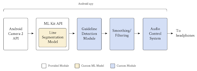 |
| Project Guideline uses Android’s built-in Camera 2 and MLKit APIs and adds custom modules to segment the guideline, detect its position and orientation, filter false signals, and send a stereo audio signal to the user in real-time. |
We faced a number of important challenges in building the preliminary Guideline system:
- System accuracy: Mobility for the blind and low vision community is a challenge in which user safety is of paramount importance. It demands a machine learning model that is capable of generating accurate and generalized segmentation results to ensure the safety of the runner in different locations and under various environmental conditions.
- System performance: In addition to addressing user safety, the system needs to be performative, efficient, and reliable. It must process at least 15 frames per second (FPS) in order to provide real-time feedback for the runner. It must also be able to run for at least 3 hours without draining the phone battery, and must work offline, without the need for internet connection should the walking/running path be in an area without data service.
- Lack of in-domain data: In order to train the segmentation model, we needed a large volume of video consisting of roads and running paths that have a yellow line on them. To generalize the model, data variety is equally as critical as data quantity, requiring video frames taken at different times of day, with different lighting conditions, under different weather conditions, at different locations, etc.
Below, we introduce solutions for each of these challenges.
Network Architecture
To meet the latency and power requirements, we built the line segmentation model on the DeepLabv3 framework, utilizing MobilenetV3-Small as the backbone, while simplifying the outputs to two classes – guideline and background.
 |
| The model takes an RGB frame and generates an output grayscale mask, representing the confidence of each pixel’s prediction. |
To increase throughput speed, we downsize the camera feed from 1920 x 1080 pixels to 513 x 513 pixels as input to the DeepLab segmentation model. To further speed-up the DeepLab model for use on mobile devices, we skipped the last up-sample layer, and directly output the 65 x 65 pixel predicted masks. These 65 x 65 pixel predicted masks are provided as input to the post processing. By minimizing the input resolution in both stages, we’re able to improve the runtime of the segmentation model and speed up post-processing.
Data Collection
To train the model, we required a large set of training images in the target domain that exhibited a variety of path conditions. Not surprisingly, the publicly available datasets were for autonomous driving use cases, with roof mounted cameras and cars driving between the lines, and were not in the target domain. We found that training models on these datasets delivered unsatisfying results due to the large domain gap. Instead, the Guideline model needed data collected with cameras worn around a person’s waist, running on top of the line, without the adversarial objects found on highways and crowded city streets.
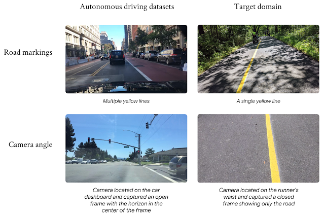 |
| The large domain gap between autonomous driving datasets and the target domain. Images on the left courtesy of the Berkeley DeepDrive dataset. |
With preexisting open-source datasets proving unhelpful for our use case, we created our own training dataset composed of the following:
- Hand-collected data: Team members temporarily placed guidelines on paved pathways using duct tape in bright colors and recorded themselves running on and around the lines at different times of the day and in different weather conditions.
- Synthetic data: The data capture efforts were complicated and severely limited due to COVID-19 restrictions. This led us to build a custom rendering pipeline to synthesize tens of thousands of images, varying the environment, weather, lighting, shadows, and adversarial objects. When the model struggled with certain conditions in real-world testing, we were able to generate specific synthetic datasets to address the situation. For example, the model originally struggled with segmenting the guideline amidst piles of fallen autumn leaves. With additional synthetic training data, we were able to correct for that in subsequent model releases.
 |
| Rendering pipeline generates synthetic images to capture a broad spectrum of environments. |
We also created a small regression dataset, which consisted of annotated samples of the most frequently seen scenarios combined with the most challenging scenarios, including tree and human shadows, fallen leaves, adversarial road markings, sunlight reflecting off the guideline, sharp turns, steep slopes, etc. We used this dataset to compare new models to previous ones and to make sure that an overall improvement in accuracy of the new model did not hide a reduction in accuracy in particularly important or challenging scenarios.
Training Procedure
We designed a three-stage training procedure and used transfer learning to overcome the limited in-domain training dataset problem. We started with a model that was pre-trained on Cityscape, and then trained the model using the synthetic images, as this dataset is larger but of lower quality. Finally, we fine-tuned the model using the limited in-domain data we collected.
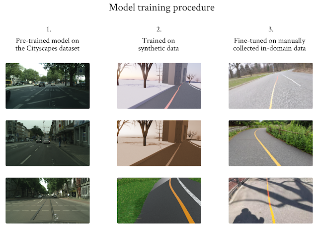 |
| Three-stage training procedure to overcome the limited data issue. Images in the left column courtesy of Cityscapes. |
Early in development, it became clear that the segmentation model’s performance suffered at the top of the image frame. As the guidelines travel further away from the camera’s point of view at the top of the frame, the lines themselves start to vanish. This causes the predicted masks to be less accurate at the top parts of the frame. To address this problem, we computed a loss value that was based on the top k pixel rows in every frame. We used this value to select those frames that included the vanishing guidelines with which the model struggled, and trained the model repeatedly on those frames. This process proved to be very helpful not only in addressing the vanishing line problem, but also for solving other problems we encountered, such as blurry frames, curved lines and line occlusion by adversarial objects.
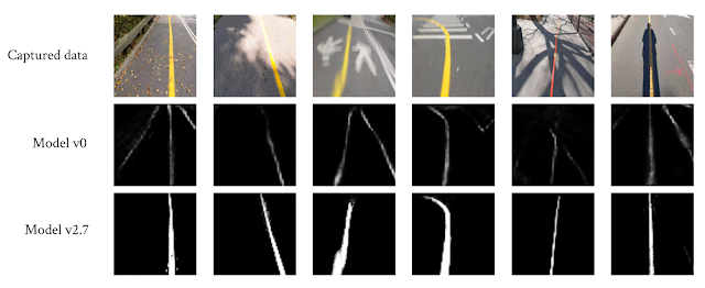 |
| The segmentation model’s accuracy and robustness continuously improved even in challenging cases. |
System Performance
Together with Tensorflow Lite and ML Kit, the end-to-end system runs remarkably fast on Pixel devices, achieving 29+ FPS on Pixel 4 XL and 20+ FPS on Pixel 5. We deployed the segmentation model entirely on DSP, running at 6 ms on Pixel 4 XL and 12 ms on Pixel 5 with high accuracy. The end-to-end system achieves 99.5% frame success rate, 93% mIoU on our evaluation dataset, and passes our regression test. These model performance metrics are incredibly important and enable the system to provide real-time feedback to the user.
What’s Next
We’re still at the beginning of our exploration, but we’re excited about our progress and what’s to come. We’re starting to collaborate with additional leading non-profit organizations that serve the blind and low vision communities to put more Guidelines in parks, schools, and public places. By painting more lines, getting direct feedback from users, and collecting more data under a wider variety of conditions, we hope to further generalize our segmentation model and improve the existing feature-set. At the same time, we are investigating new research and techniques, as well as new features and capabilities that would improve the overall system robustness and reliability.
To learn more about the project and how it came to be, read Thomas Panek’s story. If you want to help us put more Guidelines in the world, please visit goo.gle/ProjectGuideline.
Acknowledgements
Project Guideline is a collaboration across Google Research, Google Creative Lab, and the Accessibility Team. We especially would like to thank our team members: Mikhail Sirotenko, Sagar Waghmare, Lucian Lonita, Tomer Meron, Hartwig Adam, Ryan Burke, Dror Ayalon, Amit Pitaru, Matt Hall, John Watkinson, Phil Bayer, John Mernacaj, Cliff Lungaretti, Dorian Douglass, Kyndra LoCoco. We also thank Fangting Xia, Jack Sim and our other colleagues and friends from the Mobile Vision team and Guiding Eyes for the Blind.
While the robotics research community has driven recent advances that enable robots to grasp a wide range of rigid objects, less research has been devoted to developing algorithms that can handle deformable objects. One of the challenges in deformable object manipulation is that it is difficult to specify such an object’s configuration. For example, with a rigid cube, knowing the configuration of a fixed point relative to its center is sufficient to describe its arrangement in 3D space, but a single point on a piece of fabric can remain fixed while other parts shift. This makes it difficult for perception algorithms to describe the complete “state” of the fabric, especially under occlusions. In addition, even if one has a sufficiently descriptive state representation of a deformable object, its dynamics are complex. This makes it difficult to predict the future state of the deformable object after some action is applied to it, which is often needed for multi-step planning algorithms.
In “Learning to Rearrange Deformable Cables, Fabrics, and Bags with Goal-Conditioned Transporter Networks,” to appear at ICRA 2021, we release an open-source simulated benchmark, called DeformableRavens, with the goal of accelerating research into deformable object manipulation. DeformableRavens features 12 tasks that involve manipulating cables, fabrics, and bags and includes a set of model architectures for manipulating deformable objects towards desired goal configurations, specified with images. These architectures enable a robot to rearrange cables to match a target shape, to smooth a fabric to a target zone, and to insert an item in a bag. To our knowledge, this is the first simulator that includes a task in which a robot must use a bag to contain other items, which presents key challenges in enabling a robot to learn more complex relative spatial relations.
The DeformableRavens Benchmark
DeformableRavens expands our prior work on rearranging objects and includes a suite of 12 simulated tasks involving 1D, 2D, and 3D deformable structures. Each task contains a simulated UR5 arm with a mock gripper for pinch grasping, and is bundled with scripted demonstrators to autonomously collect data for imitation learning. Tasks randomize the starting state of the items within a distribution to test generality to different object configurations.
Specifying goal configurations for manipulation tasks can be particularly challenging with deformable objects. Given their complex dynamics and high-dimensional configuration spaces, goals cannot be as easily specified as a set of rigid object poses, and may involve complex relative spatial relations, such as “place the item inside the bag”. Hence, in addition to tasks defined by the distribution of scripted demonstrations, our benchmark also contains goal-conditioned tasks that are specified with goal images. For goal-conditioned tasks, a given starting configuration of objects must be paired with a separate image that shows the desired configuration of those same objects. A success for that particular case is then based on whether the robot is able to get the current configuration to be sufficiently close to the configuration conveyed in the goal image.
Goal-Conditioned Transporter Networks
To complement the goal-conditioned tasks in our simulated benchmark, we integrated goal-conditioning into our previously released Transporter Network architecture — an action-centric model architecture that works well on rigid object manipulation by rearranging deep features to infer spatial displacements from visual input. The architecture takes as input both an image of the current environment and a goal image with a desired final configuration of objects, computes deep visual features for both images, then combines the features using element-wise multiplication to condition pick and place correlations to manipulate both the rigid and deformable objects in the scene. A strength of the Transporter Network architecture is that it preserves the spatial structure of the visual images, which provides inductive biases that reformulate image-based goal conditioning into a simpler feature matching problem and improves the learning efficiency with convolutional networks.
An example task involving goal-conditioning is shown below. In order to place the green block into the yellow bag, the robot needs to learn spatial features that enable it to perform a multi-step sequence of actions to spread open the top opening of the yellow bag, before placing the block into it. After it places the block into the yellow bag, the demonstration ends in a success. If in the goal image the block were placed in the blue bag, then the demonstrator would need to put the block in the blue bag.
Results
Our results suggest that goal-conditioned Transporter Networks enable agents to manipulate deformable structures into flexibly specified configurations without test-time visual anchors for target locations. We also significantly extend prior results using Transporter Networks for manipulating deformable objects by testing on tasks with 2D and 3D deformables. Results additionally suggest that the proposed approach is more sample-efficient than alternative approaches that rely on using ground-truth pose and vertex position instead of images as input.
For example, the learned policies can effectively simulate bagging tasks, and one can also provide a goal image so that the robot must infer into which bag the item should be placed.
We encourage other researchers to check out our open-source code to try the simulated environments and to build upon this work. For more details, please check out our paper.
Future Work
This work exposes several directions for future development, including the mitigation of observed failure modes. As shown below, one failure is when the robot pulls the bag upwards and causes the item to fall out. Another is when the robot places the item on the irregular exterior surface of the bag, which causes the item to fall off. Future algorithmic improvements might allow actions that operate at a higher frequency rate, so that the robot can react in real time to counteract such failures.
Another area for advancement is to train Transporter Network-based models for deformable object manipulation using techniques that do not require expert demonstrations, such as example-based control or model-based reinforcement learning. Finally, the ongoing pandemic limited access to physical robots, so in future work we will explore the necessary ingredients to get a system working with physical bags, and to extend the system to work with different types of bags.
Acknowledgments
This research was conducted during Daniel Seita’s internship at Google’s NYC office in Summer 2020. We thank our collaborators Pete Florence, Jonathan Tompson, Erwin Coumans, Vikas Sindhwani, and Ken Goldberg.
Learning good visual and vision-language representations is critical to solving computer vision problems — image retrieval, image classification, video understanding — and can enable the development of tools and products that change people’s daily lives. For example, a good vision-language matching model can help users find the most relevant images given a text description or an image input and help tools such as Google Lens find more fine-grained information about an image.
To learn such representations, current state-of-the-art (SotA) visual and vision-language models rely heavily on curated training datasets that require expert knowledge and extensive labels. For vision applications, representations are mostly learned on large-scale datasets with explicit class labels, such as ImageNet, OpenImages, and JFT-300M. For vision-language applications, popular pre-training datasets, such as Conceptual Captions and Visual Genome Dense Captions, all require non-trivial data collection and cleaning steps, limiting the size of datasets and thus hindering the scale of the trained models. In contrast, natural language processing (NLP) models have achieved SotA performance on GLUE and SuperGLUE benchmarks by utilizing large-scale pre-training on raw text without human labels.
In “Scaling Up Visual and Vision-Language Representation Learning With Noisy Text Supervision“, to appear at ICML 2021, we propose bridging this gap with publicly available image alt-text data (written copy that appears in place of an image on a webpage if the image fails to load on a user’s screen) in order to train larger, state-of-the-art vision and vision-language models. To that end, we leverage a noisy dataset of over one billion image and alt-text pairs, obtained without expensive filtering or post-processing steps in the Conceptual Captions dataset. We show that the scale of our corpus can make up for noisy data and leads to SotA representation, and achieves strong performance when transferred to classification tasks such as ImageNet and VTAB. The aligned visual and language representations also set new SotA results on Flickr30K and MS-COCO benchmarks, even when compared with more sophisticated cross-attention models. The representations also enable zero-shot image classification and cross-modality search with complex text and text + image queries.
Creating the Dataset
Alt-texts usually provide a description of what the image is about, but the dataset is “noisy” because some text may be partly or wholly unrelated to its paired image.
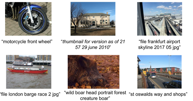 |
| Example image-text pairs randomly sampled from the training dataset of ALIGN. One clearly noisy text label is marked in italics. |
In this work, we follow the methodology of constructing the Conceptual Captions dataset to get a version of raw English alt-text data (image and alt-text pairs). While the Conceptual Captions dataset was cleaned by heavy filtering and post-processing, this work scales up visual and vision-language representation learning by relaxing most of the cleaning steps in the original work. Instead, we only apply minimal frequency-based filtering. The result is a much larger but noisier dataset of 1.8B image-text pairs.
ALIGN: A Large-scale ImaGe and Noisy-Text Embedding
For the purpose of building larger and more powerful models easily, we employ a simple dual-encoder architecture that learns to align visual and language representations of the image and text pairs. Image and text encoders are learned via a contrastive loss (formulated as normalized softmax) that pushes the embeddings of matched image-text pairs together while pushing those of non-matched image-text pairs (within the same batch) apart. The large-scale dataset makes it possible for us to scale up the model size to be as large as EfficientNet-L2 (image encoder) and BERT-large (text encoder) trained from scratch. The learned representation can be used for downstream visual and vision-language tasks.
 |
| Figure of ImageNet credit to (Krizhevsky et al. 2012) and VTAB figure credit to (Zhai et al. 2019) |
The resulting representation can be used for vision-only or vision-language task transfer. Without any fine-tuning, ALIGN powers cross-modal search – image-to-text search, text-to-image search, and even search with joint image+text queries, examples below.
 |
Evaluating Retrieval and Representation
The learned ALIGN model with BERT-Large and EfficientNet-L2 as text and image encoder backbones achieves SotA performance on multiple image-text retrieval tasks (Flickr30K and MS-COCO) in both zero-shot and fine-tuned settings, as shown below.
| Flickr30K (1K test set) R@1 | MS-COCO (5K test set) R@1 | ||||
| Setting | Model | image → text | text → image | image → text | text → image |
| Zero-shot | ImageBERT | 70.7 | 54.3 | 44.0 | 32.3 |
| UNITER | 83.6 | 68.7 | – | – | |
| CLIP | 88.0 | 68.7 | 58.4 | 37.8 | |
| ALIGN | 88.6 | 75.7 | 58.6 | 45.6 | |
| Fine-tuned | GPO | 88.7 | 76.1 | 68.1 | 52.7 |
| UNITER | 87.3 | 75.6 | 65.7 | 52.9 | |
| ERNIE-ViL | 88.1 | 76.7 | – | – | |
| VILLA | 87.9 | 76.3 | – | – | |
| Oscar | – | – | 73.5 | 57.5 | |
| ALIGN | 95.3 | 84.9 | 77.0 | 59.9 | |
| Image-text retrieval results (recall@1) on Flickr30K and MS-COCO datasets (both zero-shot and fine-tuned). ALIGN significantly outperforms existing methods including the cross-modality attention models that are too expensive for large-scale retrieval applications. |
ALIGN is also a strong image representation model. Shown below, with frozen features, ALIGN slightly outperforms CLIP and achieves a SotA result of 85.5% top-1 accuracy on ImageNet. With fine-tuning, ALIGN achieves higher accuracy than most generalist models, such as BiT and ViT, and is only worse than Meta Pseudo Labels, which requires deeper interaction between ImageNet training and large-scale unlabeled data.
| Model (backbone) | Acc@1 w/ frozen features | Acc@1 | Acc@5 |
| WSL (ResNeXt-101 32x48d) | 83.6 | 85.4 | 97.6 |
| CLIP (ViT-L/14) | 85.4 | – | – |
| BiT (ResNet152 x 4) | – | 87.54 | 98.46 |
| NoisyStudent (EfficientNet-L2) | – | 88.4 | 98.7 |
| ViT (ViT-H/14) | – | 88.55 | – |
| Meta-Pseudo-Labels (EfficientNet-L2) | – | 90.2 | 98.8 |
| ALIGN (EfficientNet-L2) | 85.5 | 88.64 | 98.67 |
| ImageNet classification results comparison with supervised training (fine-tuning). |
Zero-Shot Image Classification
Traditionally, image classification problems treat each class as independent IDs, and people have to train the classification layers with at least a few shots of labeled data per class. The class names are actually also natural language phrases, so we can naturally extend the image-text retrieval capability of ALIGN for image classification without any training data.
On the ImageNet validation dataset, ALIGN achieves 76.4% top-1 zero-shot accuracy and shows great robustness in different variants of ImageNet with distribution shifts, similar to the concurrent work CLIP. We also use the same text prompt engineering and ensembling as in CLIP.
| ImageNet | ImageNet-R | ImageNet-A | ImageNet-V2 | |
| CLIP | 76.2 | 88.9 | 77.2 | 70.1 |
| ALIGN | 76.4 | 92.2 | 75.8 | 70.1 |
| Top-1 accuracy of zero-shot classification on ImageNet and its variants. |
Application in Image Search
To illustrate the quantitative results above, we build a simple image retrieval system with the embeddings trained by ALIGN and show the top 1 text-to-image retrieval results for a handful of text queries from a 160M image pool. ALIGN can retrieve precise images given detailed descriptions of a scene, or fine-grained or instance-level concepts like landmarks and artworks. These examples demonstrate that the ALIGN model can align images and texts with similar semantics, and that ALIGN can generalize to novel complex concepts.
 |
| Image retrieval with fine-grained text queries using ALIGN’s embeddings. |
Multimodal (Image+Text) Query for Image Search
A surprising property of word vectors is that word analogies can often be solved with vector arithmetic. A common example, “king – man + woman = queen”. Such linear relationships between image and text embeddings also emerge in ALIGN.
Specifically, given a query image and a text string, we add their ALIGN embeddings together and use it to retrieve relevant images using cosine similarity, as shown below. These examples not only demonstrate the compositionality of ALIGN embeddings across vision and language domains, but also show the feasibility of searching with a multi-modal query. For instance, one could now look for the “Australia” or “Madagascar” equivalence of pandas, or turn a pair of black shoes into identically-looking beige shoes. Also, it is possible to remove objects/attributes from a scene by performing subtraction in the embedding space, shown below.
 |
| Image retrieval with image text queries. By adding or subtracting text query embedding, ALIGN retrieves relevant images. |
Social Impact and Future Work
While this work shows promising results from a methodology perspective with a simple data collection method, additional analysis of the data and the resulting model is necessary before the responsible use of the model in practice. For instance, considerations should be made towards the potential for the use of harmful text data in alt-texts to reinforce such harms. With regard to fairness, data balancing efforts may be required to prevent reinforcing stereotypes from the web data. Additional testing and training around sensitive religious or cultural items should be taken to understand and mitigate the impact from possibly mislabeled data.
Further analysis should also be taken to ensure that the demographic distribution of humans and related cultural items, such as clothing, food, and art, do not cause skewed model performance. Analysis and balancing would be required if such models will be used in production.
Conclusion
We have presented a simple method of leveraging large-scale noisy image-text data to scale up visual and vision-language representation learning. The resulting model, ALIGN, is capable of cross-modal retrieval and significantly outperforms SotA models. In visual-only downstream tasks, ALIGN is also comparable to or outperforms SotA models trained with large-scale labeled data.
Acknowledgement
We would like to thank our co-authors in Google Research: Ye Xia, Yi-Ting Chen, Zarana Parekh, Hieu Pham, Quoc V. Le, Yunhsuan Sung, Zhen Li, Tom Duerig. This work was also done with invaluable help from other colleagues from Google. We would like to thank Jan Dlabal and Zhe Li for continuous support in training infrastructure, Simon Kornblith for building the zero-shot & robustness model evaluation on ImageNet variants, Xiaohua Zhai for help on conducting VTAB evaluation, Mingxing Tan and Max Moroz for suggestions on EfficientNet training, Aleksei Timofeev for the early idea of multimodal query retrieval, Aaron Michelony and Kaushal Patel for their early work on data generation, and Sergey Ioffe, Jason Baldridge and Krishna Srinivasan for the insightful feedback and discussion.
Eye movement has been studied widely across vision science, language, and usability since the 1970s. Beyond basic research, a better understanding of eye movement could be useful in a wide variety of applications, ranging across usability and user experience research, gaming, driving, and gaze-based interaction for accessibility to healthcare. However, progress has been limited because most prior research has focused on specialized hardware-based eye trackers that are expensive and do not easily scale.
In “Accelerating eye movement research via accurate and affordable smartphone eye tracking”, published in Nature Communications, and “Digital biomarker of mental fatigue”, published in npj Digital Medicine, we present accurate, smartphone-based, ML-powered eye tracking that has the potential to unlock new research into applications across the fields of vision, accessibility, healthcare, and wellness, while additionally providing orders-of-magnitude scaling across diverse populations in the world, all using the front-facing camera on a smartphone. We also discuss the potential use of this technology as a digital biomarker of mental fatigue, which can be useful for improved wellness.
Model Overview
The core of our gaze model was a multilayer feed-forward convolutional neural network (ConvNet) trained on the MIT GazeCapture dataset. A face detection algorithm selected the face region with associated eye corner landmarks, which were used to crop the images down to the eye region alone. These cropped frames were fed through two identical ConvNet towers with shared weights. Each convolutional layer was followed by an average pooling layer. Eye corner landmarks were combined with the output of the two towers through fully connected layers. Rectified Linear Units (ReLUs) were used for all layers except the final fully connected output layer (FC6), which had no activation.
The unpersonalized gaze model accuracy was improved by fine-tuning and per-participant personalization. For the latter, a lightweight regression model was fitted to the model’s penultimate ReLU layer and participant-specific data.
Model Evaluation
To evaluate the model, we collected data from consenting study participants as they viewed dots that appeared at random locations on a blank screen. The model error was computed as the distance (in cm) between the stimulus location and model prediction. Results show that while the unpersonalized model has high error, personalization with ~30s of calibration data led to an over fourfold error reduction (from 1.92 to 0.46cm). At a viewing distance of 25-40 cm, this corresponds to 0.6-1° accuracy, a significant improvement over the 2.4-3° reported in previous work [1, 2].
Additional experiments show that the smartphone eye tracker model’s accuracy is comparable to state-of-the-art wearable eye trackers both when the phone is placed on a device stand, as well as when users hold the phone freely in their hand in a near frontal headpose. In contrast to specialized eye tracking hardware with multiple infrared cameras close to each eye, running our gaze model using a smartphone’s single front-facing RGB camera is significantly more cost effective (~100x cheaper) and scalable.
Using this smartphone technology, we were able to replicate key findings from prior eye movement research in neuroscience and psychology, including standard oculomotor tasks (to understand basic visual functioning in the brain) and natural image understanding. For example, in a simple prosaccade task, which tests a person’s ability to quickly move their eyes towards a stimulus that appears on the screen, we found that the average saccade latency (time to move the eyes) matches prior work for basic visual health (210ms versus 200-250ms). In controlled visual search tasks, we were able to replicate key findings, such as the effect of target saliency and clutter on eye movements.
For complex stimuli, such as natural images, we found that the gaze distribution (computed by aggregating gaze positions across all participants) from our smartphone eye tracker are similar to those obtained from bulky, expensive eye trackers that used highly controlled settings, such as laboratory chin rest systems. While the smartphone-based gaze heatmaps have a broader distribution (i.e., they appear more “blurred”) than hardware-based eye trackers, they are highly correlated both at the pixel level (r = 0.74) and object level (r = 0.90). These results suggest that this technology could be used to scale gaze analysis for complex stimuli such as natural and medical images (e.g., radiologists viewing MRI/PET scans).
 |
| Similar gaze distribution from our smartphone approach vs. a more expensive (100x) eye tracker (from the OSIE dataset). |
We found that smartphone gaze could also help detect difficulty with reading comprehension. Participants reading passages spent significantly more time looking within the relevant excerpts when they answered correctly. However, as comprehension difficulty increased, they spent more time looking at the irrelevant excerpts in the passage before finding the relevant excerpt that contained the answer. The fraction of gaze time spent on the relevant excerpt was a good predictor of comprehension, and strongly negatively correlated with comprehension difficulty (r = −0.72).
Digital Biomarker of Mental Fatigue
Gaze detection is an important tool to detect alertness and wellbeing, and is studied widely in medicine, sleep research, and mission-critical settings such as medical surgeries, aviation safety, etc. However, existing fatigue tests are subjective and often time-consuming. In our recent paper published in npj Digital Medicine, we demonstrated that smartphone gaze is significantly impaired with mental fatigue, and can be used to track the onset and progression of fatigue.
A simple model predicts mental fatigue reliably using just a few minutes of gaze data from participants performing a task. We validated these findings in two different experiments — using a language-independent object-tracking task and a language-dependent proofreading task. As shown below, in the object-tracking task, participants’ gaze initially follows the object’s circular trajectory, but under fatigue, their gaze shows high errors and deviations. Given the pervasiveness of phones, these results suggest that smartphone-based gaze could provide a scalable, digital biomarker of mental fatigue.
 |
| Example gaze scanpaths for a participant with no fatigue (left) versus with mental fatigue (right) as they track an object following a circular trajectory. |
 |
| The corresponding progression of fatigue scores (ground truth) and model prediction as a function of time on task. |
Beyond wellness, smartphone gaze could also provide a digital phenotype for screening or monitoring health conditions such as autism spectrum disorder, dyslexia, concussion and more. This could enable timely and early interventions, especially for countries with limited access to healthcare services.
Another area that could benefit tremendously is accessibility. People with conditions such as ALS, locked-in syndrome and stroke have impaired speech and motor ability. Smartphone gaze could provide a powerful way to make daily tasks easier by using gaze for interaction, as recently demonstrated with Look to Speak.
Ethical Considerations
Gaze research needs careful consideration, including being mindful of the correct use of such technology — applications should obtain explicit approval and fully informed consent from users for the specific task at hand. In our work, all data was collected for research purposes with users’ explicit approval and consent. In addition, users were allowed to opt out at any point and request their data to be deleted. We continue to research additional ways to ensure ML fairness and improve the accuracy and robustness of gaze technology across demographics, in a responsible, privacy-preserving way.
Conclusion
Our findings of accurate and affordable ML-powered smartphone eye tracking offer the potential for orders-of-magnitude scaling of eye movement research across disciplines (e.g., neuroscience, psychology and human-computer interaction). They unlock potential new applications for societal good, such as gaze-based interaction for accessibility, and smartphone-based screening and monitoring tools for wellness and healthcare.
Acknowledgements
This work involved collaborative efforts from a multidisciplinary team of software engineers, researchers, and cross-functional contributors. We’d like to thank all the co-authors of the papers, including our team members, Junfeng He, Na Dai, Pingmei Xu, Venky Ramachandran; interns, Ethan Steinberg, Kantwon Rogers, Li Guo, and Vincent Tseng; collaborators, Tanzeem Choudhury; and UXRs: Mina Shojaeizadeh, Preeti Talwai, and Ran Tao. We’d also like to thank Tomer Shekel, Gaurav Nemade, and Reena Lee for their contributions to this project, and Vidhya Navalpakkam for her technical leadership in initiating and overseeing this body of work.
The past decade has seen remarkable progress on automatic image captioning, a task in which a computer algorithm creates written descriptions for images. Much of the progress has come through the use of modern deep learning methods developed for both computer vision and natural language processing, combined with large scale datasets that pair images with descriptions created by people. In addition to supporting important practical applications, such as providing descriptions of images for visually impaired people, these datasets also enable investigations into important and exciting research questions about grounding language in visual inputs. For example, learning deep representations for a word like “car”, means using both linguistic and visual contexts.
Image captioning datasets that contain pairs of textual descriptions and their corresponding images, such as MS-COCO and Flickr30k, have been widely used to learn aligned image and text representations and to build captioning models. Unfortunately, these datasets have limited cross-modal associations: images are not paired with other images, captions are only paired with other captions of the same image (also called co-captions), there are image-caption pairs that match but are not labeled as a match, and there are no labels that indicate when an image-caption pair does not match. This undermines research into how inter-modality learning (connecting captions to images, for example) impacts intra-modality tasks (connecting captions to captions or images to images). This is important to address, especially because a fair amount of work on learning from images paired with text is motivated by arguments about how visual elements should inform and improve representations of language.
To address this evaluation gap, we present “Crisscrossed Captions: Extended Intramodal and Intermodal Semantic Similarity Judgments for MS-COCO“, which was recently presented at EACL 2021. The Crisscrossed Captions (CxC) dataset extends the development and test splits of MS-COCO with semantic similarity ratings for image-text, text-text and image-image pairs. The rating criteria are based on Semantic Textual Similarity, an existing and widely-adopted measure of semantic relatedness between pairs of short texts, which we extend to include judgments about images as well. In all, CxC contains human-derived semantic similarity ratings for 267,095 pairs (derived from 1,335,475 independent judgments), a massive extension in scale and detail to the 50k original binary pairings in MS-COCO’s development and test splits. We have released CxC’s ratings, along with code to merge CxC with existing MS-COCO data. Anyone familiar with MS-COCO can thus easily enhance their experiments with CxC.
Creating the CxC Dataset
If a picture is worth a thousand words, it is likely because there are so many details and relationships between objects that are generally depicted in pictures. We can describe the texture of the fur on a dog, name the logo on the frisbee it is chasing, mention the expression on the face of the person who has just thrown the frisbee, or note the vibrant red on a large leaf in a tree above the person’s head, and so on.
The CxC dataset extends the MS-COCO evaluation splits with graded similarity associations within and across modalities. MS-COCO has five captions for each image, split into 410k training, 25k development, and 25k test captions (for 82k, 5k, 5k images, respectively). An ideal extension would rate every pair in the dataset (caption-caption, image-image, and image-caption), but this is infeasible as it would require obtaining human ratings for billions of pairs.
Given that randomly selected pairs of images and captions are likely to be dissimilar, we came up with a way to select items for human rating that would include at least some new pairs with high expected similarity. To reduce the dependence of the chosen pairs on the models used to find them, we introduce an indirect sampling scheme (depicted below) where we encode images and captions using different encoding methods and compute the similarity between pairs of same modality items, resulting in similarity matrices. Images are encoded using Graph-RISE embeddings, while captions are encoded using two methods — Universal Sentence Encoder (USE) and average bag-of-words (BoW) based on GloVe embeddings. Since each MS-COCO example has five co-captions, we average the co-caption encodings to create a single representation per example, ensuring all caption pairs can be mapped to image pairs (more below on how we select intermodality pairs).
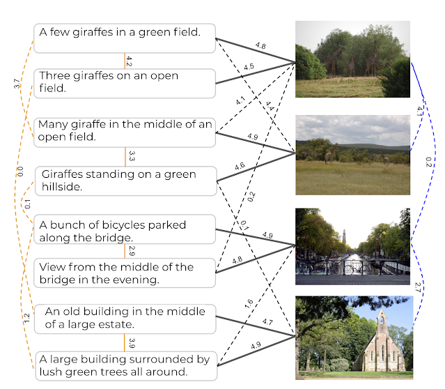
The next step of the indirect sampling scheme is to use the computed similarities of images for a biased sampling of caption pairs for human rating (and vice versa). For example, we select two captions with high computed similarities from the text similarity matrix, then take each of their images, resulting in a new pair of images that are different in appearance but similar in what they depict based on their descriptions. For example, the captions “A dog looking bashfully to the side” and “A black dog lifts its head to the side to enjoy a breeze” would have a reasonably high model similarity, so the corresponding images of the two dogs in the figure below could be selected for image similarity rating. This step can also start with two images with high computed similarities to yield a new pair of captions. We now have indirectly sampled new intramodal pairs — at least some of which are highly similar — for which we obtain human ratings.
 |
| Top: Pairs of images are picked based on their computed caption similarity. Bottom: Pairs of captions are picked based on the computed similarity of the images they describe. |
Last, we then use these new intramodal pairs and their human ratings to select new intermodal pairs for human rating. We do this by using existing image-caption pairs to link between modalities. For example, if a caption pair example ij was rated by humans as highly similar, we pick the image from example i and caption from example j to obtain a new intermodal pair for human rating. And again, we use the intramodal pairs with the highest rated similarity for sampling because this includes at least some new pairs with high similarity. Finally, we also add human ratings for all existing intermodal pairs and a large sample of co-captions.
The following table shows examples of semantic image similarity (SIS) and semantic image-text similarity (SITS) pairs corresponding to each rating, with 5 being the most similar and 0 being completely dissimilar.
 |
| Examples for each human-derived similarity score (left: 5 to 0, 5 being very similar and 0 being completely dissimilar) of image pairs based on SIS (middle) and SITS (right) tasks. Note that these examples are for illustrative purposes and are not themselves in the CxC dataset. |
Evaluation
MS-COCO supports three retrieval tasks:
- Given an image, find its matching captions out of all other captions in the evaluation set.
- Given a caption, find its corresponding image out of all other images in the evaluation set.
- Given a caption, find its other co-captions out of all other captions in the evaluation set.
MS-COCO’s pairs are incomplete because captions created for one image at times apply equally well to another, yet these associations are not captured in the dataset. CxC enhances these existing retrieval tasks with new positive pairs, and it also supports a new image-image retrieval task. With its graded similarity judgements, CxC also makes it possible to measure correlations between model and human rankings. Retrieval metrics in general focus only on positive pairs, while CxC’s correlation scores additionally account for the relative ordering of similarity and include low-scoring items (non-matches). Supporting these evaluations on a common set of images and captions makes them more valuable for understanding inter-modal learning compared to disjoint sets of caption-image, caption-caption, and image-image associations.
We ran a series of experiments to show the utility of CxC’s ratings. For this, we constructed three dual encoder (DE) models using BERT-base as the text encoder and EfficientNet-B4 as the image encoder:
- A text-text (DE_T2T) model that uses a shared text encoder for both sides.
- An image-text model (DE_I2T) that uses the aforementioned text and image encoders, and includes a layer above the text encoder to match the image encoder output.
- A multitask model (DE_I2T+T2T) trained on a weighted combination of text-text and image-text tasks.
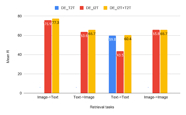 |
| CxC retrieval results — a comparison of our text-text (T2T), image-text (I2T) and multitask (I2T+T2T) dual encoder models on all the four retrieval tasks. |
From the results on the retrieval tasks, we can see that DE_I2T+T2T (yellow bar) performs better than DE_I2T (red bar) on the image-text and text-image retrieval tasks. Thus, adding the intramodal (text-text) training task helped improve the intermodal (image-text, text-image) performance. As for the other two intramodal tasks (text-text and image-image), DE_I2T+T2T shows strong, balanced performance on both of them.
 |
| CxC correlation results for the same models shown above. |
For the correlation tasks, DE_I2T performs the best on SIS and DE_I2T+T2T is the best overall. The correlation scores also show that DE_I2T performs well only on images: it has the highest SIS but has much worse STS. Adding the text-text loss to DE_I2T training (DE_I2T+T2T) produces more balanced overall performance.
The CxC dataset provides a much more complete set of relationships between and among images and captions than the raw MS-COCO image-caption pairs. The new ratings have been released and further details are in our paper. We hope to encourage the research community to push the state of the art on the tasks introduced by CxC with better models for jointly learning inter- and intra-modal representations.
Acknowledgments
The core team includes Daniel Cer, Yinfei Yang and Austin Waters. We thank Julia Hockenmaier for her inputs on CxC’s formulation, the Google Data Compute Team, especially Ashwin Kakarla and Mohd Majeed for their tooling and annotation support, Yuan Zhang, Eugene Ie for their comments on the initial versions of the paper and Daphne Luong for executive support for the data collection.
* All the images in the article have been taken from the Open Images dataset under the CC-by 4.0 license.
Sequence-to-sequence (seq2seq) models have become a favoured approach for tackling natural language generation tasks, with applications ranging from machine translation to monolingual generation tasks, such as summarization, sentence fusion, text simplification, and machine translation post-editing. However these models appear to be a suboptimal choice for many monolingual tasks, as the desired output text often represents a minor rewrite of the input text. When accomplishing such tasks, seq2seq models are both slower because they generate the output one word at a time (i.e., autoregressively), and wasteful because most of the input tokens are simply copied into the output.
Instead, text-editing models have recently received a surge of interest as they propose to predict edit operations – such as word deletion, insertion, or replacement – that are applied to the input to reconstruct the output. However, previous text-editing approaches have limitations. They are either fast (being non-autoregressive), but not flexible, because they use a limited number of edit operations, or they are flexible, supporting all possible edit operations, but slow (autoregressive). In either case, they have not focused on modeling large structural (syntactic) transformations, for example switching from active voice, “They ate steak for dinner,” to passive, “Steak was eaten for dinner.” Instead, they’ve focused on local transformations, deleting or replacing short phrases. When a large structural transformation needs to occur, they either can’t produce it or insert a large amount of new text, which is slow.
In “FELIX: Flexible Text Editing Through Tagging and Insertion”, we introduce FELIX, a fast and flexible text-editing system that models large structural changes and achieves a 90x speed-up compared to seq2seq approaches whilst achieving impressive results on four monolingual generation tasks. Compared to traditional seq2seq methods, FELIX has the following three key advantages:
- Sample efficiency: Training a high precision text generation model typically requires large amounts of high-quality supervised data. FELIX uses three techniques to minimize the amount of required data: (1) fine-tuning pre-trained checkpoints, (2) a tagging model that learns a small number of edit operations, and (3) a text insertion task that is very similar to the pre-training task.
- Fast inference time: FELIX is fully non-autoregressive, avoiding slow inference times caused by an autoregressive decoder.
- Flexible text editing: FELIX strikes a balance between the complexity of learned edit operations and flexibility in the transformations it models.
In short, FELIX is designed to derive the maximum benefit from self-supervised pre-training, being efficient in low-resource settings, with little training data.
Overview
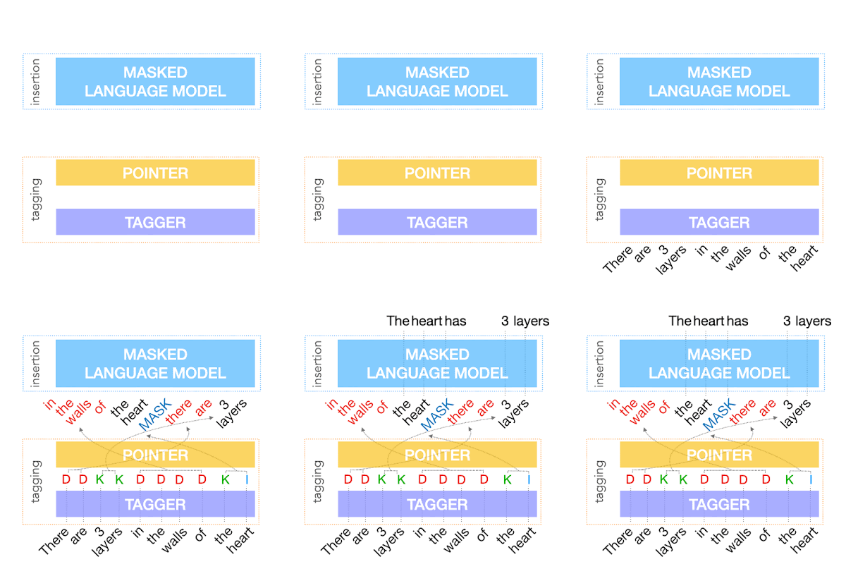
To achieve the above, FELIX decomposes the text-editing task into two sub-tasks: tagging to decide on the subset of input words and their order in the output text, and insertion, where words that are not present in the input are inserted. The tagging model employs a novel pointer mechanism, which supports structural transformations, while the insertion model is based on a Masked Language Model. Both of these models are non-autoregressive, ensuring the model is fast. A diagram of FELIX can be seen below.
The Tagging Model
The first step in FELIX is the tagging model, which consists of two components. First the tagger determines which words should be kept or deleted and where new words should be inserted. When the tagger predicts an insertion, a special MASK token is added to the output. After tagging, there is a reordering step where the pointer reorders the input to form the output, by which it is able to reuse parts of the input instead of inserting new text. The reordering step supports arbitrary rewrites, which enables modeling large changes. The pointer network is trained such that each word in the input points to the next word as it will appear in the output, as shown below.
 |
| Realization of the pointing mechanism to transform “There are 3 layers in the walls of the heart” into “the heart MASK 3 layers”. |
The Insertion Model
The output of the tagging model is the reordered input text with deleted words and MASK tokens predicted by the insertion tag. The insertion model must predict the content of MASK tokens. Because FELIX’s insertion model is very similar to the pretraining objective of BERT, it can take direct advantage of the pre-training, which is particularly advantageous when data is limited.
 |
| Example of the insertion model, where the tagger predicts two words will be inserted and the insertion model predicts the content of the MASK tokens. |
Results
We evaluated FELIX on sentence fusion, text simplification, abstractive summarization, and machine translation post-editing. These tasks vary significantly in the types of edits required and dataset sizes under which they operate. Below are the results on the sentence fusion task (i.e., merging two sentences into one), comparing FELIX against a large pre-trained seq2seq model (BERT2BERT) and a text-editing model (LaserTager), under a range of dataset sizes. We see that FELIX outperforms LaserTagger and can be trained on as little as a few hundred training examples. For the full dataset, the autoregressive BERT2BERT outperforms FELIX. However, during inference, this model takes significantly longer.
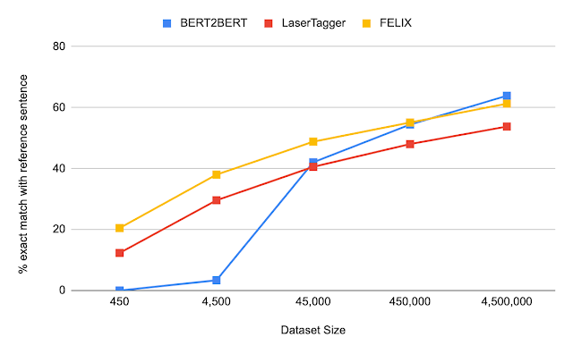 |
| A comparison of different training dataset sizes on the DiscoFuse dataset. We compare FELIX (using the best performing model) against BERT2BERT and LaserTagger. |
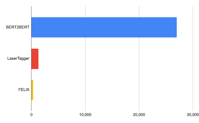 |
| Latency in milliseconds for a batch of 32 on a Nvidia Tesla P100. |
Conclusion
We have presented FELIX, which is fully non-autoregressive, providing even faster inference times, while achieving state-of-the-art results. FELIX also minimizes the amount of required training data with three techniques — fine-tuning pre-trained checkpoints, learning a small number of edit operations, and an insertion task that mimics masked language model task from the pre-training. Lastly, FELIX strikes a balance between the complexity of learned edit operations and the percentage of input-output transformations it can handle. We have open-sourced the code for FELIX and hope it will provide researchers with a faster, more efficient, and more flexible text-editing model.
Acknowledgements
This research was conducted by Jonathan Mallinson, Aliaksei Severyn (equal contribution), Eric Malmi, Guillermo Garrido. We would like to thank Aleksandr Chuklin, Daniil Mirylenka, Ryan McDonald, and Sebastian Krause for useful discussions, running early experiments and paper suggestions.


