Categories
Offsites

MaX-DeepLab: Dual-Path Transformers for End-to-End Panoptic Segmentation

Panoptic segmentation is a computer vision task that unifies semantic segmentation (assigning a class label to each pixel) and instance segmentation (detecting and segmenting each object instance). A core task for real-world applications, panoptic segmentation predicts a set of non-overlapping masks along with their corresponding class labels (i.e., category of object, like “car”, “traffic light”, “road”, etc.) and is generally accomplished using multiple surrogate sub-tasks that approximate (e.g., by using box detection methods) the goals of panoptic segmentation.

An example image and its panoptic segmentation masks from the Cityscapes dataset.
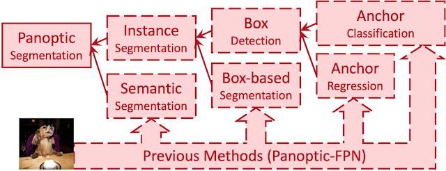
Previous methods approximate panoptic segmentation with a tree of surrogate sub-tasks.

Each surrogate sub-task in this proxy tree introduces extra manually-designed modules, such as anchor design rules, box assignment rules, non-maximum suppression (NMS), thing-stuff merging, etc. Although there are good solutions to individual surrogate sub-tasks and modules, undesired artifacts are introduced when these sub-tasks come together in a pipeline for panoptic segmentation, especially in challenging conditions (e.g., two people with similar bounding boxes will trigger NMS, resulting in a missing mask).

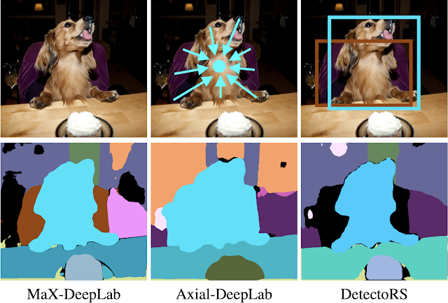
Previous efforts, such as DETR, attempted to solve some of these issues by simplifying the box detection sub-task into an end-to-end operation, which is more computationally efficient and results in fewer undesired artifacts. However, the training process still relies heavily on box detection, which does not align with the mask-based definition of panoptic segmentation. Another line of work completely removes boxes from the pipeline, which has the benefit of removing an entire surrogate sub-task along with its associated modules and artifacts. For example, Axial-DeepLab predicts pixel-wise offsets to predefined instance centers, but the surrogate sub-task it uses encounters challenges with highly deformable objects, which have a large variety of shapes (e.g., a cat), or nearby objects with close centers in the image plane, e.g. the image below of a dog seated in a chair.

When the centers of the dog and the chair are close to each other, Axial-DeepLab merges them into one object.

In “MaX-DeepLab: End-to-End Panoptic Segmentation with Mask Transformers”, to be presented at CVPR 2021, we propose the first fully end-to-end approach for the panoptic segmentation pipeline, directly predicting class-labeled masks by extending the Transformer architecture to this computer vision task. Dubbed MaX-DeepLab for extending Axial-DeepLab with a Mask Xformer, our method employs a dual-path architecture that introduces a global memory path, allowing for direct communication with any convolution layers. As a result, MaX-DeepLab shows a significant 7.1% panoptic quality (PQ) gain in the box-free regime on the challenging COCO dataset, closing the gap between box-based and box-free methods for the first time. MaX-DeepLab achieves the state-of-the-art 51.3% PQ on COCO test-dev set, without test time augmentation.

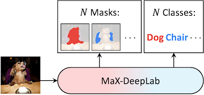
MaX-DeepLab is fully end-to-end: It predicts panoptic segmentation masks directly from images.

End-to-End Panoptic Segmentation
Inspired by DETR, our model directly predicts a set of non-overlapping masks and their corresponding semantic labels, with output masks and classes that are optimized with a PQ-style objective. Specifically, inspired by the evaluation metric, PQ, which is defined as the recognition quality (whether or not the predicted class is correct) times the segmentation quality (whether the predicted mask is correct), we define a similarity metric between two class-labeled masks in the exact same way. The model is directly trained by maximizing this similarity between ground truth masks and predicted masks via one-to-one matching. This direct modeling of panoptic segmentation enables end-to-end training and inference, removing the hand-coded priors that are necessary in existing box-based and box-free methods.

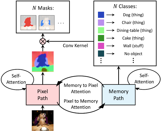
MaX-DeepLab directly predicts N masks and N classes with a CNN and a mask transformer.

Dual-Path Transformer
Instead of stacking a traditional transformer on top of a convolutional neural network (CNN), we propose a dual-path framework for combining CNNs with transformers. Specifically, we enable any CNN layer to read and write to global memory by using a dual-path transformer block. This proposed block adopts all four types of attention between the CNN-path and the memory-path, and can be inserted anywhere in a CNN, enabling communication with the global memory at any layer. MaX-DeepLab also employs a stacked-hourglass-style decoder that aggregates multi-scale features into a high resolution output. The output is then multiplied with the global memory feature, to form the mask set prediction. The classes for the masks are predicted with another branch of the mask transformer.

An overview of the dual-path transformer architecture.

Results
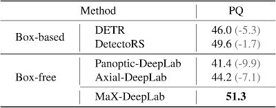
We evaluate MaX-DeepLab on one of the most challenging panoptic segmentation datasets, COCO, against both of the state-of-the-art box-free (Axial-DeepLab) and box-based (DetectoRS) methods. MaX-DeepLab, without test time augmentation, achieves the state-of-the-art result of 51.3% PQ on the test-dev set.

Comparison on COCO test-dev set.

This result surpasses Axial-DeepLab by 7.1% PQ in the box-free regime and DetectoRS by 1.7% PQ, bridging the gap between box-based and box-free methods for the first time. For a consistent comparison with DETR, we also evaluated a lightweight version of MaX-DeepLab that matches the number of parameters and computations of DETR. The lightweight MaX-DeepLab outperforms DETR by 3.3% PQ on the val set and 3.0% PQ on the test-dev set. In addition, we performed extensive ablation studies and analyses on our end-to-end formulation, model scaling, dual-path architectures, and loss functions. Also the extra-long training schedule of DETR is not necessary for MaX-DeepLab.

As an example in the figure below, MaX-DeepLab correctly segments a dog sitting on a chair. Axial-DeepLab relies on a surrogate sub-task of regressing object center offsets. It fails because the centers of the dog and the chair are close to each other. DetectoRS classifies object bounding boxes, instead of masks, as a surrogate sub-task. It filters out the chair mask because the chair bounding box has a low confidence.

A case study for MaX-DeepLab and state-of-the-art box-free and box-based methods.

Another example shows how MaX-DeepLab correctly segments images with challenging conditions.

MaX-DeepLab correctly segments the overlapping zebras. This case is also challenging for other methods since the zebras have similar bounding boxes and nearby object centers. (credit & license)

Conclusion
We have shown for the first time that panoptic segmentation can be trained end-to-end. MaX-DeepLab directly predicts masks and classes with a mask transformer, removing the need for many hand-designed priors such as object bounding boxes, thing-stuff merging, etc. Equipped with a PQ-style loss and a dual-path transformer, MaX-DeepLab achieves the state-of-the-art result on the challenging COCO dataset, closing the gap between box-based and box-free methods.

Acknowledgements
We are thankful to our co-authors, Yukun Zhu, Hartwig Adam, and Alan Yuille. We also thank Maxwell Collins, Sergey Ioffe, Jiquan Ngiam, Siyuan Qiao, Chen Wei, Jieneng Chen, and the Mobile Vision team for the support and valuable discussions.

Categories
Offsites

Multi-Task Robotic Reinforcement Learning at Scale

For general-purpose robots to be most useful, they would need to be able to perform a range of tasks, such as cleaning, maintenance and delivery. But training even a single task (e.g., grasping) using offline reinforcement learning (RL), a trial and error learning method where the agent uses training previously collected data, can take thousands of robot-hours, in addition to the significant engineering needed to enable autonomous operation of a large-scale robotic system. Thus, the computational costs of building general-purpose everyday robots using current robot learning methods becomes prohibitive as the number of tasks grows.

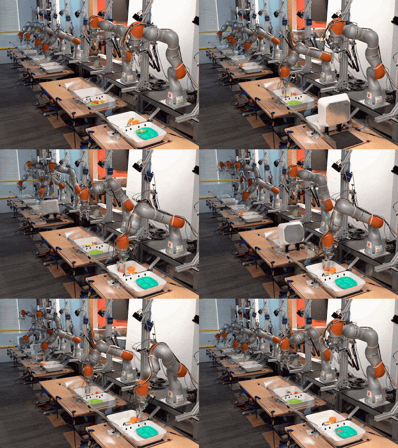
Multi-task data collection across multiple robots where different robots collect data for different tasks.

In other large-scale machine learning domains, such as natural language processing and computer vision, a number of strategies have been applied to amortize the effort of learning over multiple skills. For example, pre-training on large natural language datasets can enable few- or zero-shot learning of multiple tasks, such as question answering and sentiment analysis. However, because robots collect their own data, robotic skill learning presents a unique set of opportunities and challenges. Automating this process is a large engineering endeavour, and effectively reusing past robotic data collected by different robots remains an open problem.

Today we present two new advances for robotic RL at scale, MT-Opt, a new multi-task RL system for automated data collection and multi-task RL training, and Actionable Models, which leverages the acquired data for goal-conditioned RL. MT-Opt introduces a scalable data-collection mechanism that is used to collect over 800,000 episodes of various tasks on real robots and demonstrates a successful application of multi-task RL that yields ~3x average improvement over baseline. Additionally, it enables robots to master new tasks quickly through use of its extensive multi-task dataset (new task fine-tuning in <1 day of data collection). Actionable Models enables learning in the absence of specific tasks and rewards by training an implicit model of the world that is also an actionable robotic policy. This drastically increases the number of tasks the robot can perform (via visual goal specification) and enables more efficient learning of downstream tasks.

Large-Scale Multi-Task Data Collection System
The cornerstone for both MT-Opt and Actionable Models is the volume and quality of training data. To collect diverse, multi-task data at scale, users need a way to specify tasks, decide for which tasks to collect the data, and finally, manage and balance the resulting dataset. To that end, we create a scalable and intuitive multi-task success detector using data from all of the chosen tasks. The multi-task success is trained using supervised learning to detect the outcome of a given task and it allows users to quickly define new tasks and their rewards. When this success detector is being applied to collect data, it is periodically updated to accommodate distribution shifts caused by various real-world factors, such as varying lighting conditions, changing background surroundings, and novel states that the robots discover.

Second, we simultaneously collect data for multiple distinct tasks across multiple robots by using solutions to easier tasks to effectively bootstrap learning of more complex tasks. This allows training of a policy for the harder tasks and improves the data collected for them. As such, the amount of per-task data and the number of successful episodes for each task grows over time. To further improve the performance, we focus data collection on underperforming tasks, rather than collecting data uniformly across tasks.

This system collected 9600 robot hours of data (from 57 continuous data collection days on seven robots). However, while this data collection strategy was effective at collecting data for a large number of tasks, the success rate and data volume was imbalanced between tasks.

Learning with MT-Opt
We address the data collection imbalance by transferring data across tasks and re-balancing the per-task data. The robots generate episodes that are labelled as success or failure for each task and are then copied and shared across other tasks. The balanced batch of episodes is then sent to our multi-task RL training pipeline to train the MT-Opt policy.

Data sharing and task re-balancing strategy used by MT-Opt. The robots generate episodes which then get labelled as success or failure for the current task and are then shared across other tasks.

MT-Opt uses Q-learning, a popular RL method that learns a function that estimates the future sum of rewards, called the Q-function. The learned policy then picks the action that maximizes this learned Q-function. For multi-task policy training, we specify the task as an extra input to a large Q-learning network (inspired by our previous work on large-scale single-task learning with QT-Opt) and then train all of the tasks simultaneously with offline RL using the entire multi-task dataset. In this way, MT-Opt is able to train on a wide variety of skills that include picking specific objects, placing them into various fixtures, aligning items on a rack, rearranging and covering objects with towels, etc.

Compared to single-task baselines, MT-Opt performs similarly on the tasks that have the most data and significantly improves performance on underrepresented tasks. So, for a generic lifting task, which has the most supporting data, MT-Opt achieved an 89% success rate (compared to 88% for QT-Opt) and achieved a 50% average success rate across rare tasks, compared to 1% with a single-task QT-Opt baseline and 18% using a naïve, multi-task QT-Opt baseline. Using MT-Opt not only enables zero-shot generalization to new but similar tasks, but also can quickly (in about 1 day of data collection on seven robots) be fine-tuned to new, previously unseen tasks. For example, when applied to an unseen towel-covering task, the system achieved a zero-shot success rate of 92% for towel-picking and 79% for object-covering, which wasn’t present in the original dataset.

Example tasks that MT-Opt is able to learn, such as instance and indiscriminate grasping, chasing, placing, aligning and rearranging.

<!–

Example tasks that MT-Opt is able to learn, such as instance and indiscriminate grasping, chasing, placing, aligning and rearranging.

–>

Towel-covering task that was not present in the original dataset. We fine-tune MT-Opt on this novel task in 1 day to achieve a high (>90%) success rate.

Learning with Actionable Models
While supplying a rigid definition of tasks facilitates autonomous data collection for MT-Opt, it limits the number of learnable behaviors to a fixed set. To enable learning a wider range of tasks from the same data, we use goal-conditioned learning, i.e., learning to reach given goal configurations of a scene in front of the robot, which we specify with goal images. In contrast to explicit model-based methods that learn predictive models of future world observations, or approaches that employ online data collection, this approach learns goal-conditioned policies via offline model-free RL.

To learn to reach any goal state, we perform hindsight relabeling of all trajectories and sub-sequences in our collected dataset and train a goal-conditioned Q-function in a fully offline manner (in contrast to learning online using a fixed set of success examples as in recursive classification). One challenge in this setting is the distributional shift caused by learning only from “positive” hindsight relabeled examples. This we address by employing a conservative strategy to minimize Q-values of unseen actions using artificial negative actions. Furthermore, to enable reaching temporary-extended goals, we introduce a technique for chaining goals across multiple episodes.

Actionable Models relabel sub-sequences with all intermediate goals and regularize Q-values with artificial negative actions.

Training with Actionable Models allows the system to learn a large repertoire of visually indicated skills, such as object grasping, container placing and object rearrangement. The model is also able to generalize to novel objects and visual objectives not seen in the training data, which demonstrates its ability to learn general functional knowledge about the world. We also show that downstream reinforcement learning tasks can be learned more efficiently by either fine-tuning a pre-trained goal-conditioned model or through a goal-reaching auxiliary objective during training.

Example tasks (specified by goal-images) that our Actionable Model is able to learn.

Conclusion
The results of both MT-Opt and Actionable Models indicate that it is possible to collect and then learn many distinct tasks from large diverse real-robot datasets within a single model, effectively amortizing the cost of learning across many skills. We see this an important step towards general robot learning systems that can be further scaled up to perform many useful services and serve as a starting point for learning downstream tasks.

This post is based on two papers, “MT-Opt: Continuous Multi-Task Robotic Reinforcement Learning at Scale” and “Actionable Models: Unsupervised Offline Reinforcement Learning of Robotic Skills,” with additional information and videos on the project websites for MT-Opt and Actionable Models.

Acknowledgements
This research was conducted by Dmitry Kalashnikov, Jake Varley, Yevgen Chebotar, Ben Swanson, Rico Jonschkowski, Chelsea Finn, Sergey Levine, Yao Lu, Alex Irpan, Ben Eysenbach, Ryan Julian and Ted Xiao. We’d like to give special thanks to Josh Weaver, Noah Brown, Khem Holden, Linda Luu and Brandon Kinman for their robot operation support; Anthony Brohan for help with distributed learning and testing infrastructure; Tom Small for help with videos and project media; Julian Ibarz, Kanishka Rao, Vikas Sindhwani and Vincent Vanhoucke for their support; Tuna Toksoz and Garrett Peake for improving the bin reset mechanisms; Satoshi Kataoka, Michael Ahn, and Ken Oslund for help with the underlying control stack, and the rest of the Robotics at Google team for their overall support and encouragement. All the above contributions were incredibly enabling for this research.

Categories
Offsites

Presenting the iGibson Challenge on Interactive and Social Navigation

Computer vision has significantly advanced over the past decade thanks to large-scale benchmarks, such as ImageNet for image classification or COCO for object detection, which provide vast datasets and criteria for evaluating models. However, these traditional benchmarks evaluate passive tasks in which the emphasis is on perception alone, whereas more recent computer vision research has tackled active tasks, which require both perception and action (often called “embodied AI”).

The First Embodied AI Workshop, co-organized by Google at CVPR 2020, hosted several benchmark challenges for active tasks, including the Stanford and Google organized Sim2Real Challenge with iGibson, which provided a real-world setup to test navigation policies trained in photo-realistic simulation environments. An open-source setup in the challenge enabled the community to train policies in simulation, which could then be run in repeatable real world navigation experiments, enabling the evaluation of the “sim-to-real gap” — the difference between simulation and the real world. Many research teams submitted solutions during the pandemic, which were run safely by challenge organizers on real robots, with winners presenting their results virtually at the workshop.

This year, Stanford and Google are proud to announce a new version of the iGibson Challenge on Interactive and Social Navigation, one of the 10 active visual challenges affiliated with the Second Embodied AI Workshop at CVPR 2021. This year’s Embodied AI Workshop is co-organized by Google and nine other research organizations, and explores issues such as simulation, sim-to-real transfer, visual navigation, semantic mapping and change detection, object rearrangement and restoration, auditory navigation, and following instructions for navigation and interaction tasks. In addition, this year’s interactive and social iGibson challenge explores interactive navigation and social navigation — how robots can learn to interact with people and objects in their environments — by combining the iGibson simulator, the Google Scanned Objects Dataset, and simulated pedestrians within realistic human environments.

New Challenges in Navigation
Active perception tasks are challenging, as they require both perception and actions in response. For example, point navigation involves navigating through mapped space, such as driving robots over kilometers in human-friendly buildings, while recognizing and avoiding obstacles. Similarly object navigation involves looking for objects in buildings, requiring domain invariant representations and object search behaviors. Additionally, visual language instruction navigation involves navigating through buildings based on visual images and commands in natural language. These problems become even harder in a real-world environment, where robots must be able to handle a variety of physical and social interactions that are much more dynamic and challenging to solve. In this year’s iGibson Challenge, we focus on two of those settings:

  • Interactive Navigation: In a cluttered environment, an agent navigating to a goal must physically interact with objects to succeed. For example, an agent should recognize that a shoe can be pushed aside, but that an end table should not be moved and a sofa cannot be moved.
  • Social Navigation: In a crowded environment in which people are also moving about, an agent navigating to a goal must move politely around the people present with as little disruption as possible.

New Features of the iGibson 2021 Dataset
To facilitate research into techniques that address these problems, the iGibson Challenge 2021 dataset provides simulated interactive scenes for training. The dataset includes eight fully interactive scenes derived from real-world apartments, and another seven scenes held back for testing and evaluation.

iGibson provides eight fully interactive scenes derived from real-world apartments.

To enable interactive navigation, these scenes are populated with small objects drawn from the Google Scanned Objects Dataset, a dataset of common household objects scanned in 3D for use in robot simulation and computer vision research, licensed under a Creative Commons license to give researchers the freedom to use them in their research.

The Google Scanned Objects Dataset contains 3D models of many common objects.

The challenge is implemented in Stanford’s open-source iGibson simulation platform, a fast, interactive, photorealistic robotic simulator with physics based on Bullet. For this year’s challenge, iGibson has been expanded with fully interactive environments and pedestrian behaviors based on the ORCA crowd simulation algorithm.

iGibson environments include ORCA crowd simulations and movable objects.

Participating in the Challenge
The iGibson Challenge has launched and its leaderboard is open in the Dev phase, in which participants are encouraged to submit robotic control to the development leaderboard, where they will be tested on the Interactive and Social Navigation challenges on our holdout dataset. The Test phase opens for teams to submit final solutions on May 16th and closes on May 31st, with the winner demo scheduled for June 20th, 2021. For more details on participating, please check out the iGibson Challenge Page.

Acknowledgements
We’d like to thank our colleagues at at the Stanford Vision and Learning Lab (SVL) for working with us to advance the state of interactive and social robot navigation, including Chengshu Li, Claudia Pérez D’Arpino, Fei Xia, Jaewoo Jang, Roberto Martin-Martin and Silvio Savarese. At Google, we would like to thank Aleksandra Faust, Anelia Angelova, Carolina Parada, Edward Lee, Jie Tan, Krista Reyman and the rest of our collaborators on mobile robotics. We would also like to thank our co-organizers on the Embodied AI Workshop, including AI2, Facebook, Georgia Tech, Intel, MIT, SFU, Stanford, UC Berkeley, and University of Washington.

Categories
Offsites

Monster Mash: A Sketch-Based Tool for Casual 3D Modeling and Animation

3D computer animation is a time-consuming and highly technical medium — to complete even a single animated scene requires numerous steps, like modeling, rigging and animating, each of which is itself a sub-discipline that can take years to master. Because of its complexity, 3D animation is generally practiced by teams of skilled specialists and is inaccessible to almost everyone else, despite decades of advances in technology and tools. With the recent development of tools that facilitate game character creation and game balance, a natural question arises: is it possible to democratize the 3D animation process so it’s accessible to everyone?

To explore this concept, we start with the observation that most forms of artistic expression have a casual mode: a classical guitarist might jam without any written music, a trained actor could ad-lib a line or two while rehearsing, and an oil painter can jot down a quick gesture drawing. What these casual modes have in common is that they allow an artist to express a complete thought quickly and intuitively without fear of making a mistake. This turns out to be essential to the creative process — when each sketch is nearly effortless, it is possible to iteratively explore the space of possibilities far more effectively.

In this post, we describe Monster Mash, an open source tool presented at SIGGRAPH Asia 2020 that allows experts and amateurs alike to create rich, expressive, deformable 3D models from scratch — and to animate them — all in a casual mode, without ever having to leave the 2D plane. With Monster Mash, the user sketches out a character, and the software automatically converts it to a soft, deformable 3D model that the user can immediately animate by grabbing parts of it and moving them around in real time. There is also an online demo, where you can try it out for yourself.

Creating a walk cycle using Monster Mash. Step 1: Draw a character. Step 2: Animate it.

Creating a 2D Sketch
The insight that makes this casual sketching approach possible is that many 3D models, particularly those of organic forms, can be described by an ordered set of overlapping 2D regions. This abstraction makes the complex task of 3D modeling much easier: the user creates 2D regions by drawing their outlines, then the algorithm creates a 3D model by stitching the regions together and inflating them. The result is a simple and intuitive user interface for sketching 3D figures.

For example, suppose the user wants to create a 3D model of an elephant. The first step is to draw the body as a closed stroke (a). Then the user adds strokes to depict other body parts such as legs (b). Drawing those additional strokes as open curves provides a hint to the system that they are meant to be smoothly connected with the regions they overlap. The user can also specify that some new parts should go behind the existing ones by drawing them with the right mouse button (c), and mark other parts as symmetrical by double-clicking on them (d). The result is an ordered list of 2D regions.

Steps in creating a 2D sketch of an elephant.

Stitching and Inflation
To understand how a 3D model is created from these 2D regions, let’s look more closely at one part of the elephant. First, the system identifies where the leg must be connected to the body (a) by finding the segment (red) that completes the open curve. The system cuts the body’s front surface along that segment, and then stitches the front of the leg together with the body (b). It then inflates the model into 3D by solving a modified form of Poisson’s equation to produce a surface with a rounded cross-section (c). The resulting model (d) is smooth and well-shaped, but because all of the 3D parts are rooted in the drawing plane, they may intersect each other, resulting in a somewhat odd-looking “elephant”. These intersections will be resolved by the deformation system.

Illustration of the details of the stitching and inflation process. The schematic illustrations (b, c) are cross-sections viewed from the elephant’s front.

Layered Deformation
At this point we just have a static model — we need to give the user an easy way to pose the model, and also separate the intersecting parts somehow. Monster Mash’s layered deformation system, based on the well-known smooth deformation method as-rigid-as-possible (ARAP), solves both of these problems at once. What’s novel about our layered “ARAP-L” approach is that it combines deformation and other constraints into a single optimization framework, allowing these processes to run in parallel at interactive speed, so that the user can manipulate the model in real time.

The framework incorporates a set of layering and equality constraints, which move body parts along the z axis to prevent them from visibly intersecting each other. These constraints are applied only at the silhouettes of overlapping parts, and are dynamically updated each frame.

In steps (d) through (h) above, ARAP-L transforms a model from one with intersecting 3D parts to one with the depth ordering specified by the user. The layering constraints force the leg’s silhouette to stay in front of the body (green), and the body’s silhouette to stay behind the leg (yellow). Equality constraints (red) seal together the loose boundaries between the leg and the body.

Meanwhile, in a separate thread of the framework, we satisfy point constraints to make the model follow user-defined control points (described in the section below) in the xy-plane. This ARAP-L method allows us to combine modeling, rigging, deformation, and animation all into a single process that is much more approachable to the non-specialist user.

The model deforms to match the point constraints (red dots) while the layering constraints prevent the parts from visibly intersecting.

Animation
To pose the model, the user can create control points anywhere on the model’s surface and move them. The deformation system converges over multiple frames, which gives the model’s movement a soft and floppy quality, allowing the user to intuitively grasp its dynamic properties — an essential prerequisite for kinesthetic learning.

Because the effect of deformations converges over multiple frames, our system lends 3D models a soft and dynamic quality.

To create animation, the system records the user’s movements in real time. The user can animate one control point, then play back that movement while recording additional control points. In this way, the user can build up a complex action like a walk by layering animation, one body part at a time. At every stage of the animation process, the only task required of the user is to move points around in 2D, a low-risk workflow meant to encourage experimentation and play.

Conclusion
We believe this new way of creating animation is intuitive and can thus help democratize the field of computer animation, encouraging novices who would normally be unable to try it on their own as well as experts who often require fast iteration under tight deadlines. Here you can see a few of the animated characters that have been created using Monster Mash. Most of these were created in a matter of minutes.

A selection of animated characters created using Monster Mash. The original hand-drawn outline used to create each 3D model is visible as an inset above each character.

All of the code for Monster Mash is available as open source, and you can watch our presentation and read our paper from SIGGRAPH Asia 2020 to learn more. We hope this software will make creating 3D animations more broadly accessible. Try out the online demo and see for yourself!

Acknowledgements
Monster Mash is the result of a collaboration between Google Research, Czech Technical University in Prague, ETH Zürich, and the University of Washington. Key contributors include Marek Dvorožňák, Daniel Sýkora, Cassidy Curtis, Brian Curless, Olga Sorkine-Hornung, and David Salesin. We are also grateful to Hélène Leroux, Neth Nom, David Murphy, Samuel Leather, Pavla Sýkorová, and Jakub Javora for participating in the early interactive sessions.

Categories
Offsites

Announcing the 2021 Research Scholar Program Recipients

In March 2020 we introduced the Research Scholar Program, an effort focused on developing collaborations with new professors and encouraging the formation of long-term relationships with the academic community. In November we opened the inaugural call for proposals for this program, which was received with enthusiastic interest from faculty who are working on cutting edge research across many research areas in computer science, including machine learning, human computer interaction, health research, systems and more.

Today, we are pleased to announce that in this first year of the program we have granted 77 awards, which included 86 principal investigators representing 15+ countries and over 50 universities. Of the 86 award recipients, 43% identify as an historically marginalized group within technology. Please see the full list of 2021 recipients on our web page, as well as in the list below.

We offer our congratulations to this year’s recipients, and look forward to seeing what they achieve!

Algorithms and Optimization
Alexandros Psomas, Purdue University
Auction Theory Beyond Independent, Quasi-Linear Bidders
Julian Shun, Massachusetts Institute of Technology
Scalable Parallel Subgraph Finding and Peeling Algorithms
Mary Wootters, Stanford University
The Role of Redundancy in Algorithm Design
Pravesh K. Kothari, Carnegie Mellon University
Efficient Algorithms for Robust Machine Learning
Sepehr Assadi, Rutgers University
Graph Clustering at Scale via Improved Massively Parallel Algorithms

Augmented Reality and Virtual Reality
Srinath Sridhar, Brown University
Perception and Generation of Interactive Objects

Geo
Miriam E. Marlier, University of California, Los Angeles
Mapping California’s Compound Climate Hazards in Google Earth Engine
Suining He, The University of Connecticut
Fairness-Aware and Cross-Modality Traffic Learning and Predictive Modeling for Urban Smart Mobility Systems

Human Computer Interaction
Arvind Satyanarayan, Massachusetts Institute of Technology
Generating Semantically Rich Natural Language Captions for Data Visualizations to Promote Accessibility
Dina EL-Zanfaly, Carnegie Mellon University
In-the-making: An intelligence mediated collaboration system for creative practices
Katharina Reinecke, University of Washington
Providing Science-Backed Answers to Health-related Questions in Google Search
Misha Sra, University of California, Santa Barbara
Hands-free Game Controller for Quadriplegic Individuals
Mohsen Mosleh, University of Exeter Business School
Effective Strategies to Debunk False Claims on Social Media: A large-scale digital field experiments approach
Tanushree Mitra, University of Washington
Supporting Scalable Value-Sensitive Fact-Checking through Human-AI Intelligence

Health Research
Catarina Barata, Instituto Superior Técnico, Universidade de Lisboa
DeepMutation – A CNN Model To Predict Genetic Mutations In Melanoma Patients
Emma Pierson, Cornell Tech, the Jacobs Institute, Technion-Israel Institute of Technology, and Cornell University
Using cell phone mobility data to reduce inequality and improve public health
Jasmine Jones, Berea College
Reachout: Co-Designing Social Connection Technologies for Isolated Young Adults
Mojtaba Golzan, University of Technology Sydney, Jack Phu, University of New South Wales
Autonomous Grading of Dynamic Blood Vessel Markers in the Eye using Deep Learning
Serena Yeung, Stanford University
Artificial Intelligence Analysis of Surgical Technique in the Operating Room

Machine Learning and data mining
Aravindan Vijayaraghavan, Northwestern University, Sivaraman Balakrishnan, Carnegie Mellon University
Principled Approaches for Learning with Test-time Robustness
Cho-Jui Hsieh, University of California, Los Angeles
Scalability and Tunability for Neural Network Optimizers
Golnoosh Farnadi, University of Montreal, HEC Montreal/MILA
Addressing Algorithmic Fairness in Decision-focused Deep Learning
Harrie Oosterhuis, Radboud University
Search and Recommendation Systems that Learn from Diverse User Preferences
Jimmy Ba, University of Toronto
Model-based Reinforcement Learning with Causal World Models
Nadav Cohen, Tel-Aviv University
A Dynamical Theory of Deep Learning
Nihar Shah, Carnegie Mellon University
Addressing Unfairness in Distributed Human Decisions
Nima Fazeli, University of Michigan
Semi-Implicit Methods for Deformable Object Manipulation
Qingyao Ai, University of Utah
Metric-agnostic Ranking Optimization
Stefanie Jegelka, Massachusetts Institute of Technology
Generalization of Graph Neural Networks under Distribution Shifts
Virginia Smith, Carnegie Mellon University
A Multi-Task Approach for Trustworthy Federated Learning

Mobile
Aruna Balasubramanian, State University of New York – Stony Brook
AccessWear: Ubiquitous Accessibility using Wearables
Tingjun Chen, Duke University
Machine Learning- and Optical-enabled Mobile Millimeter-Wave Networks

Machine Perception
Amir Patel, University of Cape Town
WildPose: 3D Animal Biomechanics in the Field using Multi-Sensor Data Fusion
Angjoo Kanazawa, University of California, Berkeley
Practical Volumetric Capture of People and Scenes
Emanuele Rodolà, Sapienza University of Rome
Fair Geometry: Toward Algorithmic Debiasing in Geometric Deep Learning
Minchen Wei, The Hong Kong Polytechnic University
Accurate Capture of Perceived Object Colors for Smart Phone Cameras
Mohsen Ali, Information Technology University of the Punjab, Pakistan, Izza Aftab, Information Technology University of the Punjab, Pakistan
Is Economics From Afar Domain Generalizable?
Vineeth N Balasubramanian, Indian Institute of Technology Hyderabad
Bridging Perspectives of Explainability and Adversarial Robustness
Xin Yu, University of Technology Sydney, Linchao Zhu, University of Technology Sydney
Sign Language Translation in the Wild

Networking
Aurojit Panda, New York University
Bertha: Network APIs for the Programmable Network Era
Cristina Klippel Dominicini, Instituto Federal do Espirito Santo
Polynomial Key-based Architecture for Source Routing in Network Fabrics
Noa Zilberman, University of Oxford
Exposing Vulnerabilities in Programmable Network Devices
Rachit Agarwal, Cornell University
Designing Datacenter Transport for Terabit Ethernet

Natural Language Processing
Danqi Chen, Princeton University
Improving Training and Inference Efficiency of NLP Models
Derry Tanti Wijaya, Boston University, Anietie Andy, University of Pennsylvania
Exploring the evolution of racial biases over time through framing analysis
Eunsol Choi, University of Texas at Austin
Answering Information Seeking Questions In The Wild
Kai-Wei Chang, University of California, Los Angeles
Certified Robustness to against language differences in Cross-Lingual Transfer
Mohohlo Samuel Tsoeu, University of Cape Town
Corpora collection and complete natural language processing of isiXhosa, Sesotho and South African Sign languages
Natalia Diaz Rodriguez, University of Granada (Spain) + ENSTA, Institut Polytechnique Paris, Inria. Lorenzo Baraldi, University of Modena and Reggio Emilia
SignNet: Towards democratizing content accessibility for the deaf by aligning multi-modal sign representations

Other Research Areas
John Dickerson, University of Maryland – College Park, Nicholas Mattei, Tulane University
Fairness and Diversity in Graduate Admissions
Mor Nitzan, Hebrew University
Learning representations of tissue design principles from single-cell data
Nikolai Matni, University of Pennsylvania
Robust Learning for Safe Control

Privacy
Foteini Baldimtsi, George Mason University
Improved Single-Use Anonymous Credentials with Private Metabit
Yu-Xiang Wang, University of California, Santa Barbara
Stronger, Better and More Accessible Differential Privacy with autodp

Quantum Computing
Ashok Ajoy, University of California, Berkeley
Accelerating NMR spectroscopy with a Quantum Computer
John Nichol, University of Rochester
Coherent spin-photon coupling
Jordi Tura i Brugués, Leiden University
RAGECLIQ – Randomness Generation with Certification via Limited Quantum Devices
Nathan Wiebe, University of Toronto
New Frameworks for Quantum Simulation and Machine Learning
Philipp Hauke, University of Trento
ProGauge: Protecting Gauge Symmetry in Quantum Hardware
Shruti Puri, Yale University
Surface Code Co-Design for Practical Fault-Tolerant Quantum Computing

Structured data, extraction, semantic graph, and database management
Abolfazl Asudeh, University Of Illinois, Chicago
An end-to-end system for detecting cherry-picked trendlines
Eugene Wu, Columbia University
Interactive training data debugging for ML analytics
Jingbo Shang, University of California, San Diego
Structuring Massive Text Corpora via Extremely Weak Supervision

Security
Chitchanok Chuengsatiansup, The University of Adelaide, Markus Wagner, The University of Adelaide
Automatic Post-Quantum Cryptographic Code Generation and Optimization
Elette Boyle, IDC Herzliya, Israel
Cheaper Private Set Intersection via Advances in “Silent OT”
Joseph Bonneau, New York University
Zeroizing keys in secure messaging implementations
Yu Feng , University of California, Santa Barbara, Yuan Tian, University of Virginia
Exploit Generation Using Reinforcement Learning

Software engineering and programming languages
Kelly Blincoe, University of Auckland
Towards more inclusive software engineering practices to retain women in software engineering
Fredrik Kjolstad, Stanford University
Sparse Tensor Algebra Compilation to Domain-Specific Architectures
Milos Gligoric, University of Texas at Austin
Adaptive Regression Test Selection
Sarah E. Chasins, University of California, Berkeley
If you break it, you fix it: Synthesizing program transformations so that library maintainers can make breaking changes

Systems
Adwait Jog, College of William & Mary
Enabling Efficient Sharing of Emerging GPUs
Heiner Litz, University of California, Santa Cruz
Software Prefetching Irregular Memory Access Patterns
Malte Schwarzkopf, Brown University
Privacy-Compliant Web Services by Construction
Mehdi Saligane, University of Michigan
Autonomous generation of Open Source Analog & Mixed Signal IC
Nathan Beckmann, Carnegie Mellon University
Making Data Access Faster and Cheaper with Smarter Flash Caches
Yanjing Li, University of Chicago
Resilient Accelerators for Deep Learning Training Tasks

Categories
Offsites

Python TensorFlow Tutorial – Build a Neural Network

Updated for TensorFlow 2

Google’s TensorFlow has been a hot topic in deep learning recently.  The open source software, designed to allow efficient computation of data flow graphs, is especially suited to deep learning tasks.  It is designed to be executed on single or multiple CPUs and GPUs, making it a good option for complex deep learning tasks.  In its most recent incarnation – version 1.0 – it can even be run on certain mobile operating systems.  This introductory tutorial to TensorFlow will give an overview of some of the basic concepts of TensorFlow in Python.  These will be a good stepping stone to building more complex deep learning networks, such as Convolution Neural Networks, natural language models, and Recurrent Neural Networks in the package.  We’ll be creating a simple three-layer neural network to classify the MNIST dataset.  This tutorial assumes that you are familiar with the basics of neural networks, which you can get up to scratch with in the neural networks tutorial if required.  To install TensorFlow, follow the instructions here. The code for this tutorial can be found in this site’s GitHub repository.  Once you’re done, you also might want to check out a higher level deep learning library that sits on top of TensorFlow called Keras – see my Keras tutorial.

First, let’s have a look at the main ideas of TensorFlow.

1.0 TensorFlow graphs

TensorFlow is based on graph based computation – “what on earth is that?”, you might say.  It’s an alternative way of conceptualising mathematical calculations.  Consider the following expression $a = (b + c) * (c + 2)$.  We can break this function down into the following components:

begin{align}
d &= b + c \
e &= c + 2 \
a &= d * e
end{align}

Now we can represent these operations graphically as:

TensorFlow tutorial - simple computational graph

Simple computational graph

This may seem like a silly example – but notice a powerful idea in expressing the equation this way: two of the computations ($d=b+c$ and $e=c+2$) can be performed in parallel.  By splitting up these calculations across CPUs or GPUs, this can give us significant gains in computational times.  These gains are a must for big data applications and deep learning – especially for complicated neural network architectures such as Convolutional Neural Networks (CNNs) and Recurrent Neural Networks (RNNs).  The idea behind TensorFlow is to the ability to create these computational graphs in code and allow significant performance improvements via parallel operations and other efficiency gains.

We can look at a similar graph in TensorFlow below, which shows the computational graph of a three-layer neural network.

TensorFlow tutorial - data flow graph

TensorFlow data flow graph

The animated data flows between different nodes in the graph are tensors which are multi-dimensional data arrays.  For instance, the input data tensor may be 5000 x 64 x 1, which represents a 64 node input layer with 5000 training samples.  After the input layer, there is a hidden layer with rectified linear units as the activation function.  There is a final output layer (called a “logit layer” in the above graph) that uses cross-entropy as a cost/loss function.  At each point we see the relevant tensors flowing to the “Gradients” block which finally flows to the Stochastic Gradient Descent optimizer which performs the back-propagation and gradient descent.

Here we can see how computational graphs can be used to represent the calculations in neural networks, and this, of course, is what TensorFlow excels at.  Let’s see how to perform some basic mathematical operations in TensorFlow to get a feel for how it all works.

2.0 A Simple TensorFlow example

So how can we make TensorFlow perform the little example calculation shown above – $a = (b + c) * (c + 2)$? First, there is a need to introduce TensorFlow variables.  The code below shows how to declare these objects:

import tensorflow as tf
# create TensorFlow variables
const = tf.Variable(2.0, name="const")
b = tf.Variable(2.0, name='b')
c = tf.Variable(1.0, name='c')

As can be observed above, TensorFlow variables can be declared using the tf.Variable function.  The first argument is the value to be assigned to the variable. The second is an optional name string which can be used to label the constant/variable – this is handy for when you want to do visualizations.  TensorFlow will infer the type of the variable from the initialized value, but it can also be set explicitly using the optional dtype argument.  TensorFlow has many of its own types like tf.float32, tf.int32 etc.

The objects assigned to the Python variables are actually TensorFlow tensors. Thereafter, they act like normal Python objects – therefore, if you want to access the tensors you need to keep track of the Python variables. In previous versions of TensorFlow, there were global methods of accessing the tensors and operations based on their names. This is no longer the case.

To examine the tensors stored in the Python variables, simply call them as you would a normal Python variable. If we do this for the “const” variable, you will see the following output:

<tf.Variable ‘const:0’ shape=() dtype=float32, numpy=2.0>

This output gives you a few different pieces of information – first, is the name ‘const:0’ which has been assigned to the tensor. Next is the data type, in this case, a TensorFlow float 32 type. Finally, there is a “numpy” value. TensorFlow variables in TensorFlow 2 can be converted easily into numpy objects. Numpy stands for Numerical Python and is a crucial library for Python data science and machine learning. If you don’t know Numpy, what it is, and how to use it, check out this site. The command to access the numpy form of the tensor is simply .numpy() – the use of this method will be shown shortly.

Next, some calculation operations are created:

# now create some operations
d = tf.add(b, c, name='d')
e = tf.add(c, const, name='e')
a = tf.multiply(d, e, name='a')

Note that d and e are automatically converted to tensor values upon the execution of the operations. TensorFlow has a wealth of calculation operations available to perform all sorts of interactions between tensors, as you will discover as you progress through this book.  The purpose of the operations shown above are pretty obvious, and they instantiate the operations b + c, c + 2.0, and d * e. However, these operations are an unwieldy way of doing things in TensorFlow 2. The operations below are equivalent to those above:

d = b + c
e = c + 2
a = d * e

To access the value of variable a, one can use the .numpy() method as shown below:

print(f”Variable a is {a.numpy()}”)

The computational graph for this simple example can be visualized by using the TensorBoard functionality that comes packaged with TensorFlow. This is a great visualization feature and is explained more in this post. Here is what the graph looks like in TensorBoard:

TensorFlow tutorial - simple graph

Simple TensorFlow graph

The larger two vertices or nodes, b and c, correspond to the variables. The smaller nodes correspond to the operations, and the edges between the vertices are the scalar values emerging from the variables and operations.

The example above is a trivial example – what would this look like if there was an array of b values from which an array of equivalent a values would be calculated? TensorFlow variables can easily be instantiated using numpy variables, like the following:

b = tf.Variable(np.arange(0, 10), name='b')

Calling b shows the following:

<tf.Variable ‘b:0’ shape=(10,) dtype=int32, numpy=array([0, 1, 2, 3, 4, 5, 6, 7, 8, 9])>

Note the numpy value of the tensor is an array. Because the numpy variable passed during the instantiation is a range of int32 values, we can’t add it directly to c as c is of float32 type. Therefore, the tf.cast operation, which changes the type of a tensor, first needs to be utilized like so:

d = tf.cast(b, tf.float32) + c

Running the rest of the previous operations, using the new b tensor, gives the following value for a:

Variable a is [ 3.  6.  9. 12. 15. 18. 21. 24. 27. 30.]

In numpy, the developer can directly access slices or individual indices of an array and change their values directly. Can the same be done in TensorFlow 2? Can individual indices and/or slices be accessed and changed? The answer is yes, but not quite as straight-forwardly as in numpy. For instance, if b was a simple numpy array, one could easily execute the following b[1] = 10 – this would change the value of the second element in the array to the integer 10.

b[1].assign(10)

This will then flow through to a like so:

Variable a is [ 3. 33.  9. 12. 15. 18. 21. 24. 27. 30.]

The developer could also run the following, to assign a slice of b values:

b[6:9].assign([10, 10, 10])

A new tensor can also be created by using the slice notation:

f = b[2:5]

The explanations and code above show you how to perform some basic tensor manipulations and operations. In the section below, an example will be presented where a neural network is created using the Eager paradigm in TensorFlow 2. It will show how to create a training loop, perform a feed-forward pass through a neural network and calculate and apply gradients to an optimization method.

3.0 A Neural Network Example

In this section, a simple three-layer neural network build in TensorFlow is demonstrated.  In following chapters more complicated neural network structures such as convolution neural networks and recurrent neural networks are covered.  For this example, though, it will be kept simple.

In this example, the MNIST dataset will be used that is packaged as part of the TensorFlow installation. This MNIST dataset is a set of 28×28 pixel grayscale images which represent hand-written digits.  It has 60,000 training rows, 10,000 testing rows, and 5,000 validation rows. It is a very common, basic, image classification dataset that is used in machine learning.

The data can be loaded by running the following:

from tensorflow.keras.datasets import mnist
(x_train, y_train), (x_test, y_test) = mnist.load_data()

As can be observed, the Keras MNIST data loader returns Python tuples corresponding to the training and test set respectively (Keras is another deep learning framework, now tightly integrated with TensorFlow, as mentioned earlier). The data sizes of the tuples defined above are:

  • x_train: (60,000 x 28 x 28)
  • y_train: (60,000)
  • x_test: (10,000 x 28 x 28)
  • y_test: (10,000)

The x data is the image information – 60,000 images of 28 x 28 pixels size in the training set. The images are grayscale (i.e black and white) with maximum values, specifying the intensity of whites, of 255. The x data will need to be scaled so that it resides between 0 and 1, as this improves training efficiency. The y data is the matching image labels – signifying what digit is displayed in the image. This will need to be transformed to “one-hot” format.

When using a standard, categorical cross-entropy loss function (this will be shown later), a one-hot format is required when training classification tasks, as the output layer of the neural network will have the same number of nodes as the total number of possible classification labels. The output node with the highest value is considered as a prediction for that corresponding label. For instance, in the MNIST task, there are 10 possible classification labels – 0 to 9. Therefore, there will be 10 output nodes in any neural network performing this classification task. If we have an example output vector of [0.01, 0.8, 0.25, 0.05, 0.10, 0.27, 0.55, 0.32, 0.11, 0.09], the maximum value is in the second position / output node, and therefore this corresponds to the digit “1”. To train the network to produce this sort of outcome when the digit “1” appears, the loss needs to be calculated according to the difference between the output of the network and a “one-hot” array of the label 1. This one-hot array looks like [0, 1, 0, 0, 0, 0, 0, 0, 0, 0].

This conversion is easily performed in TensorFlow, as will be demonstrated shortly when the main training loop is covered.

One final thing that needs to be considered is how to extract the training data in batches of samples. The function below can handle this:

def get_batch(x_data, y_data, batch_size):
    idxs = np.random.randint(0, len(y_data), batch_size)
    return x_data[idxs,:,:], y_data[idxs]

As can be observed in the code above, the data to be batched i.e. the x and y data is passed to this function along with the batch size. The first line of the function generates a random vector of integers, with random values between 0 and the length of the data passed to the function. The number of random integers generated is equal to the batch size. The x and y data are then returned, but the return data is only for those random indices chosen. Note, that this is performed on numpy array objects – as will be shown shortly, the conversion from numpy arrays to tensor objects will be performed “on the fly” within the training loop.

There is also the requirement for a loss function and a feed-forward function, but these will be covered shortly.

# Python optimisation variables
epochs = 10
batch_size = 100

# normalize the input images by dividing by 255.0
x_train = x_train / 255.0
x_test = x_test / 255.0
# convert x_test to tensor to pass through model (train data will be converted to
# tensors on the fly)
x_test = tf.Variable(x_test)

First, the number of training epochs and the batch size are created – note these are simple Python variables, not TensorFlow variables. Next, the input training and test data, x_train and x_test, are scaled so that their values are between 0 and 1. Input data should always be scaled when training neural networks, as large, uncontrolled, inputs can heavily impact the training process. Finally, the test input data, x_test is converted into a tensor. The random batching process for the training data is most easily performed using numpy objects and functions. However, the test data will not be batched in this example, so the full test input data set x_test is converted into a tensor.

The next step is to setup the weight and bias variables for the three-layer neural network.  There are always L – 1 number of weights/bias tensors, where L is the number of layers.  These variables are defined in the code below:

# now declare the weights connecting the input to the hidden layer
W1 = tf.Variable(tf.random.normal([784, 300], stddev=0.03), name='W1')
b1 = tf.Variable(tf.random.normal([300]), name='b1')
# and the weights connecting the hidden layer to the output layer
W2 = tf.Variable(tf.random.normal([300, 10], stddev=0.03), name='W2')
b2 = tf.Variable(tf.random.normal([10]), name='b2')

The weight and bias variables are initialized using the tf.random.normal function – this function creates tensors of random numbers, drawn from a normal distribution. It allows the developer to specify things like the standard deviation of the distribution from which the random numbers are drawn.

Note the shape of the variables. The W1 variable is a [784, 300] tensor – the 784 nodes are the size of the input layer. This size comes from the flattening of the input images – if we have 28 rows and 28 columns of pixels, flattening these out gives us 1 row or column of 28 x 28 = 784 values.  The 300 in the declaration of W1 is the number of nodes in the hidden layer. The W2 variable is a [300, 10] tensor, connecting the 300-node hidden layer to the 10-node output layer. In each case, a name is given to the variable for later viewing in TensorBoard – the TensorFlow visualization package. The next step in the code is to create the computations that occur within the nodes of the network. If the reader recalls, the computations within the nodes of a neural network are of the following form:

$$z = Wx + b$$

$$h=f(z)$$

Where W is the weights matrix, x is the layer input vector, b is the bias and f is the activation function of the node. These calculations comprise the feed-forward pass of the input data through the neural network. To execute these calculations, a dedicated feed-forward function is created:

def nn_model(x_input, W1, b1, W2, b2):
    # flatten the input image from 28 x 28 to 784
    x_input = tf.reshape(x_input, (x_input.shape[0], -1))
    x = tf.add(tf.matmul(tf.cast(x_input, tf.float32), W1), b1)
    x = tf.nn.relu(x)
    logits = tf.add(tf.matmul(x, W2), b2)
    return logits

Examining the first line, the x_input data is reshaped from (batch_size, 28, 28) to (batch_size, 784) – in other words, the images are flattened out. On the next line, the input data is then converted to tf.float32 type using the TensorFlow cast function. This is important – the x­_input data comes in as tf.float64 type, and TensorFlow won’t perform a matrix multiplication operation (tf.matmul) between tensors of different data types. This re-typed input data is then matrix-multiplied by W1 using the TensorFlow matmul function (which stands for matrix multiplication). Then the bias b1 is added to this product. On the line after this, the ReLU activation function is applied to the output of this line of calculation. The ReLU function is usually the best activation function to use in deep learning – the reasons for this are discussed in this post.

The output of this calculation is then multiplied by the final set of weights W2, with the bias b2 added. The output of this calculation is titled logits. Note that no activation function has been applied to this output layer of nodes (yet). In machine/deep learning, the term “logits” refers to the un-activated output of a layer of nodes.

The reason no activation function has been applied to this layer is that there is a handy function in TensorFlow called tf.nn.softmax_cross_entropy_with_logits. This function does two things for the developer – it applies a softmax activation function to the logits, which transforms them into a quasi-probability (i.e. the sum of the output nodes is equal to 1). This is a common activation function to apply to an output layer in classification tasks. Next, it applies the cross-entropy loss function to the softmax activation output. The cross-entropy loss function is a commonly used loss in classification tasks. The theory behind it is quite interesting, but it won’t be covered in this book – a good summary can be found here. The code below applies this handy TensorFlow function, and in this example,  it has been nested in another function called loss_fn:

def loss_fn(logits, labels):
    cross_entropy = tf.reduce_mean(tf.nn.softmax_cross_entropy_with_logits(labels=labels,
                                                                              logits=logits))
    return cross_entropy

The arguments to softmax_cross_entropy_with_logits are labels and logits. The logits argument is supplied from the outcome of the nn_model function. The usage of this function in the main training loop will be demonstrated shortly. The labels argument is supplied from the one-hot y values that are fed into loss_fn during the training process. The output of the softmax_cross_entropy_with_logits function will be the output of the cross-entropy loss value for each sample in the batch. To train the weights of the neural network, the average cross-entropy loss across the samples needs to be minimized as part of the optimization process. This is calculated by using the tf.reduce_mean function, which, unsurprisingly, calculates the mean of the tensor supplied to it.

The next step is to define an optimizer function. In many examples within this book, the versatile Adam optimizer will be used. The theory behind this optimizer is interesting, and is worth further examination (such as shown here) but won’t be covered in detail within this post. It is basically a gradient descent method, but with sophisticated averaging of the gradients to provide appropriate momentum to the learning. To define the optimizer, which will be used in the main training loop, the following code is run:

# setup the optimizer
optimizer = tf.keras.optimizers.Adam()

The Adam object can take a learning rate as input, but for the present purposes, the default value is used.

3.1 Training the network

Now that the appropriate functions, variables and optimizers have been created, it is time to define the overall training loop. The training loop is shown below:

total_batch = int(len(y_train) / batch_size)
for epoch in range(epochs):
    avg_loss = 0
    for i in range(total_batch):
        batch_x, batch_y = get_batch(x_train, y_train, batch_size=batch_size)
        # create tensors
        batch_x = tf.Variable(batch_x)
        batch_y = tf.Variable(batch_y)
        # create a one hot vector
        batch_y = tf.one_hot(batch_y, 10)
        with tf.GradientTape() as tape:
            logits = nn_model(batch_x, W1, b1, W2, b2)
            loss = loss_fn(logits, batch_y)
        gradients = tape.gradient(loss, [W1, b1, W2, b2])
        optimizer.apply_gradients(zip(gradients, [W1, b1, W2, b2]))
        avg_loss += loss /..
Categories
Offsites

A2C Advantage Actor Critic in TensorFlow 2

In a previous post, I gave an introduction to Policy Gradient reinforcement learning. Policy gradient-based reinforcement learning relies on using neural networks to learn an action policy for the control of agents in an environment. This is opposed to controlling agents based on neural network estimations of a value-based function, such as the Q value in deep Q learning. However, there are problems with straight Monte-Carlo based methods of policy gradient learning as covered in the previously mentioned policy gradient post. In particular, one significant problem is a high variance in the learning. This problem can be solved by a process called baselining, with the most effective baselining method being the Advantage Actor Critic method or A2c. In this post, I’ll review the theory of the A2c method, and demonstrate how to build an A2c algorithm in TensorFlow 2.

All code shown in this tutorial can be found at this site’s Github repository, in the ac2_tf2_cartpole.py file.

A quick recap of some important concepts

In the A2C algorithm, notice the title “Advantage Actor” – this refers first to the actor, the part of the neural network that is used to determine the actions of the agent. The “advantage” is a concept that expresses the relative benefit of taking a certain action at time t ($a_t$) from a certain state $s_t$. Note that it is not the “absolute” benefit, but the “relative” benefit. This will become clearer when I discuss the concept of “value”. The advantage is expressed as:

$$A(s_t, a_t) = Q(s_t, a_t) – V(s_t)$$

The Q value (discussed in other posts, for instance here, here and here) is the expected future rewards of taking action $a_t$ from state $s_t$. The value $V(s_t)$ is the expected value of the agent being in that state and operating under a certain action policy $pi$. It can be expressed as:

$$V^{pi}(s) = mathbb{E} left[sum_{i=1}^T gamma^{i-1}r_{i}right]$$

Here $mathbb{E}$ is the expectation operator, and the value $V^{pi}(s)$ can be read as the expected value of future discounted rewards that will be gathered by the agent, operating under a certain action policy $pi$. So, the Q value is the expected value of taking a certain action from the current state, whereas V is the expected value of simply being in the current state, under a certain action policy.

The advantage then is the relative benefit of taking a certain action from the current state. It’s kind of like a normalized Q value. For example, let’s consider the last state in a game, where after the next action the game ends. There are three possible actions from this state, with rewards of (51, 50, 49). Let’s also assume that the action selection policy $pi$ is simply random, so there is an equal chance of any of the three actions being selected. The value of this state, then, is 50 ((51+50+49) / 3). If the first action is randomly selected (reward=51), the Q value is 51. However, the advantage is only equal to 1 (Q-V = 51-50). As can be observed and as stated above, the advantage is a kind of normalized or relative Q value.

Why is this important? If we are using Q values in some way to train our action-taking policy, in the example above the first action would send a “signal” or contribution of 51 to the gradient optimizer, which may be significant enough to push the parameters of the neural network significantly in a certain direction. However, given the other two actions possible from this state also have a high reward (50 and 49), the signal or contribution is really higher than it should be – it is not that much better to take action 1 instead of action 3. Therefore, Q values can be a source of high variance in the training process, and it is much better to use the normalized or baseline Q values i.e. the advantage, in training. For more discussion of Q, values, and advantages, see my post on dueling Q networks.

Policy gradient reinforcement learning and its problems

In a previous post, I presented the policy gradient reinforcement learning algorithm. For details on this algorithm, please consult that post. However, the A2C algorithm shares important similarities with the PG algorithm, and therefore it is necessary to recap some of the theory. First, it has to be recalled that PG-based algorithms involve a neural network that directly outputs estimates of the probability distribution of the best next action to take in a given state. So, for instance, if we have an environment with 4 possible actions, the output from the neural network could be something like [0.5, 0.25, 0.1, 0.15], with the first action being currently favored. In the PG case, then, the neural network is the direct instantiation of the policy of the agent $pi_{theta}$ – where this policy is controlled by the parameters of the neural network $theta$. This is opposed to Q based RL algorithms, where the neural network estimates the Q value in a given state for each possible action. In these algorithms, the action policy is generally an epsilon-greedy policy, where the best action is that action with the highest Q value (with some random choices involved to improve exploration).

The gradient of the loss function for the policy gradient algorithm is as follows:

$$nabla_theta J(theta) sim left(sum_{t=0}^{T-1} log P_{pi_{theta}}(a_t|s_t)right)left(sum_{t’= t + 1}^{T} gamma^{t’-t-1} r_{t’} right)$$

Note that the term:

$$G_t = left(sum_{t’= t + 1}^{T} gamma^{t’-t-1} r_{t’} right)$$

Is just the discounted sum of the rewards onwards from state $s_t$. In other words, it is an estimate of the true value function $V^{pi}(s)$. Remember that in the PG algorithm, the network can only be trained after each full episode, and this is because of the term above. Therefore, note that the $G_t$ term above is an estimate of the true value function as it is based on only a single trajectory of the agent through the game.

Now, because it is based on samples of reward trajectories, which aren’t “normalized” or baselined in any way, the PG algorithm suffers from variance issues, resulting in slower and more erratic training progress. A better solution is to replace the $G_t$ function above with the Advantage – $A(s_t, a_t)$, and this is what the Advantage-Actor Critic method does.

The A2C algorithm

Replacing the $G_t$ function with the advantage, we come up with the following gradient function which can be used in training the neural network:

$$nabla_theta J(theta) sim left(sum_{t=0}^{T-1} log P_{pi_{theta}}(a_t|s_t)right)A(s_t, a_t)$$

Now, as shown above, the advantage is:

$$A(s_t, a_t) = Q(s_t, a_t) – V(s_t)$$

However, using Bellman’s equation, the Q value can be expressed purely in terms of the rewards and the value function:

$$Q(s_t, a_t) = mathbb{E}left[r_{t+1} + gamma V(s_{t+1})right]$$

Therefore, the advantage can now be estimated as:

$$A(s_t, a_t) = r_{t+1} + gamma V(s_{t+1}) – V(s_t)$$

As can be seen from the above, there is a requirement to be able to estimate the value function V. We could estimate it by running our agents through full episodes, in the same way we did in the policy gradient method. However, it would be better to be able to just collect batches of game-steps and train whenever the batch buffer was full, rather than having to wait for an episode to finish. That way, the agent could actually learn “on-the-go” during the middle of an episode/game.

So, do we build another neural network to estimate V? We could have two networks, one to learn the policy and produce actions, and another to estimate the state values. A more efficient solution is to create one network, but with two output channels, and this is how the A2C method is outworked. The figure below shows the network architecture for an A2C neural network:

A2C architecture

A2C architecture

This architecture is based on an A2C method that takes game images as the state input, hence the convolutional neural network layers at the beginning of the network (for more on CNNs, see my post here). This network architecture also resembles the Dueling Q network architecture (see my Dueling Q post). The point to note about the architecture above is that most of the network is shared, with a late bifurcation between the policy part and the value part. The outputs $P(s, a_i)$ are the action probabilities of the policy (generated from the neural network) – $P(a_t|s_t)$. The other output channel is the value estimation – a scalar output which is the predicted value of state s – $V(s)$. The two dense channels disambiguate the policy and the value outputs from the front-end of the neural network.

In this example, we’ll just be demonstrating the A2C algorithm on the Cartpole OpenAI Gym environment which doesn’t require a visual state input (i.e. a set of pixels as the input to the NN), and therefore the two output channels will simply share some dense layers, rather than a series of CNN layers.

The A2C loss functions

There are actually three loss values that need to be calculated in the A2C algorithm. Each of these losses is in practice given a weighting, and then they are summed together (with the entropy loss having a negative sign, see below).

The Critic loss

The loss function of the Critic i.e. the value estimating output of the neural network $V(s)$, needs to be trained so that it predicts more and more closely the actual value of the state. As shown before, the value of a state is calculated as:

$$V^{pi}(s) = mathbb{E} left[sum_{i=1}^T gamma^{i-1}r_{i}right]$$

So $V^{pi}(s)$ is the expected value of the discounted future rewards obtained by outworking a trajectory through the game based on a certain operating policy $pi$. We can therefore compare the predicted $V(s)$ at each state in the game, and the actual sampled discounted rewards that were gathered, and the difference between the two is the Critic loss. In this example, we’ll use a mean squared error function as the loss function, between the discounted rewards and the predicted values ($(V(s) – DR)^2$).

Now, given that, under the A2C algorithm, we collect state, action and reward tuples until a batch buffer is filled, how are we meant to figure out this discounted rewards sum? Let’s say we progress 3 states through a game, and we collect:

$(V(s_0), r_0), (V(s_1), r_1), (V(s_2), r_2)$

For the first Critic loss, we could calculate it as:

$$MSE(V(s_0), r_0 + gamma r_1 + gamma^2 r_2)$$

But that is missing all the following rewards $r_3, r_4, …., r_n$ until the game terminates. We didn’t have this problem in the Policy Gradient method, because in that method, we made sure a full run through the game had completed before training the neural network. In the A2c method, we use a trick called bootstrapping. To replace all the discounted $r_3, r_4, …., r_n$ values, we get the network to estimate the value for state 3, $V(s_3)$, and this will be an estimate for all the discounted future rewards beyond that point in the game. So, for the first Critic loss, we would have:

$$MSE(V(s_0), r_0 + gamma r_1 + gamma^2 r_2 + gamma^3 V(s_3))$$

Where $V(s_3)$ is a bootstrapped estimate of the value of the next state $s_3$.

This will be explained more in the code-walkthrough to follow.

The Actor loss

The second loss function needs to train the Actor (i.e. the action policy). Recall that the advantage weighted policy loss is:

$$nabla_theta J(theta) sim left(sum_{t=0}^{T-1} log P_{pi_{theta}}(a_t|s_t)right)A(s_t, a_t)$$

Let’s start with the advantage – $A(s_t, a_t) = r_{t+1} + gamma V(s_{t+1}) – V(s_t)$

This is simply the bootstrapped discounted rewards minus the predicted state values $V(s_t)$ that we gathered up while playing the game. So calculating the advantage is quite straight-forward, once we have the bootstrapped discounted rewards, as will be seen in the code walk-through shortly.

Now, with regards to the $log P_{pi_{theta}}(a_t|s_t)$ statement, in this instance, we can just calculate the log of the softmax probability estimate for whatever action was taken. So, for instance, if in state 1 ($s_1$) the network softmax output produces {0.1, 0.9} (for a 2-action environment), and the second action was actually taken by the agent, we would want to calculate log(0.9). We can make use of the TensorFlow-Keras SparseCategoricalCrossEntropy calculation, which takes the action as an integer, and this specifies which softmax output value to apply the log to. So in this example, y_pred = [1] and y_target = [0.1, 0.9] and the answer would be -log(0.9) = 0.105.

Another handy feature with the SpareCategoricalCrossEntropy loss in Keras is that it can be called with a “sample_weight” argument. This basically multiplies the log calculation with a value. So, in this example, we can supply the advantages as the sample weights, and it will calculate  $nabla_theta J(theta) sim left(sum_{t=0}^{T-1} log P_{pi_{theta}}(a_t|s_t)right)A(s_t, a_t)$ for us. This will be shown below, but the call will look like:

policy_loss = sparse_ce(actions, policy_logits, sample_weight=advantages)

Entropy loss

In many implementations of the A2c algorithm, another loss term is subtracted – the entropy loss. Entropy is a measure, broadly speaking, of randomness. The higher the entropy, the more random the state of affairs, the lower the entropy, the more ordered the state of affairs. In the case of A2c, entropy is calculated on the softmax policy action ($P(a_t|s_t)$) output of the neural network. Let’s go back to our two action example from above. In the case of a probability output of {0.1, 0.9} for the two possible actions, this is an ordered, less-random selection of actions. In other words, there will be a consistent selection of action 2, and only rarely will action 1 be taken. The entropy formula is:

$$E = -sum p(x) log(p(x))$$

So in this case, the entropy of that output would be 0.325. However, if the probability output was instead {0.5, 0.5}, the entropy would be 0.693. The 50-50 action probability distribution will produce more random actions, and therefore the entropy is higher.

By subtracting the entropy calculation from the total loss (or giving the entropy loss a negative sign), it encourages more randomness and therefore more exploration. The A2c algorithm can have a tendency of converging on particular actions, so this subtraction of the entropy encourages a better exploration of alternative actions, though making the weighting on this component of the loss too large can also reduce training performance.

Again, we can use an already existing Keras loss function to calculate the entropy. The Keras categorical cross-entropy performs the following calculation:

Keras output of cross-entropy loss function

Keras output of cross-entropy loss function

If we just pass in the probability outputs as both target and output to this function, then it will calculate the entropy for us. This will be shown in the code below.

The total loss

The total loss function for the A2C algorithm is:

Loss = Actor Loss + Critic Loss * CRITIC_WEIGHT – Entropy Loss * ENTROPY_WEIGHT

A common value for the critic weight is 0.5, and the entropy weight is usually quite low (i.e. on the order of 0.01-0.001), though these hyperparameters can be adjusted and experimented with depending on the environment and network.

Implementing A2C in TensorFlow 2

In the following section, I will provide a walk-through of some code to implement the A2C methodology in TensorFlow 2. The code for this can be found at this site’s Github repository, in the ac2_tf2_cartpole.py file.

First, we perform the usual imports, set some constants, initialize the environment and finally create the neural network model which instantiates the A2C architecture:

import tensorflow as tf
from tensorflow import keras
import numpy as np
import gym
import datetime as dt

STORE_PATH = '/Users/andrewthomas/Adventures in ML/TensorFlowBook/TensorBoard/A2CCartPole'
CRITIC_LOSS_WEIGHT = 0.5
ACTOR_LOSS_WEIGHT = 1.0
ENTROPY_LOSS_WEIGHT = 0.05
BATCH_SIZE = 64
GAMMA = 0.95

env = gym.make("CartPole-v0")
state_size = 4
num_actions = env.action_space.n


class Model(keras.Model):
    def __init__(self, num_actions):
        super().__init__()
        self.num_actions = num_actions
        self.dense1 = keras.layers.Dense(64, activation='relu',
                                         kernel_initializer=keras.initializers.he_normal())
        self.dense2 = keras.layers.Dense(64, activation='relu',
                                         kernel_initializer=keras.initializers.he_normal())
        self.value = keras.layers.Dense(1)
        self.policy_logits = keras.layers.Dense(num_actions)

    def call(self, inputs):
        x = self.dense1(inputs)
        x = self.dense2(x)
        return self.value(x), self.policy_logits(x)

    def action_value(self, state):
        value, logits = self.predict_on_batch(state)
        action = tf.random.categorical(logits, 1)[0]
        return action, value

As can be seen, for this example I have set the critic, actor and entropy loss weights to 0.5, 1.0 and 0.05 respectively. Next the environment is setup, and then the model class is created.

This class inherits from keras.Model, which enables it to be integrated into the streamlined Keras methods of training and evaluating (for more information, see this Keras tutorial). In the initialization of the class, we see that 2 dense layers have been created, with 64 nodes in each. Then a value layer with one output is created, which evaluates $V(s)$, and finally the policy layer output with a size equal to the number of available actions. Note that this layer produces logits only, the softmax function which creates pseudo-probabilities ($P(a_t, s_t)$) will be applied within the various TensorFlow functions, as will be seen.

Next, the call function is defined – this function is run whenever a state needs to be “run” through the model, to produce a value and policy logits output. The Keras model API will use this function in its predict functions and also its training functions. In this function, it can be observed that the input is passed through the two common dense layers, and then the function returns first the value output, then the policy logits output.

The next function is the action_value function. This function is called upon when an action needs to be chosen from the model. As can be seen, the first step of the function is to run the predict_on_batch Keras model API function. This function just runs the model.call function defined above. The output is both the values and the policy logits. An action is then selected by randomly choosing an action based on the action probabilities. Note that tf.random.categorical takes as input logits, not softmax outputs. The next function, outside of the Model class, is the function that calculates the critic loss:

def critic_loss(discounted_rewards, predicted_values):
    return keras.losses.mean_squared_error(discounted_rewards, predicted_values) * CRITIC_LOSS_WEIGHT

As explained above, the critic loss comprises of the mean squared error between the discounted rewards (which is calculated in another function, soon to be discussed) and the values predicted from the value output of the model (which are accumulated in a list during the agent’s trajectory through the game).

The following function shows the actor loss function:

def actor_loss(combined, policy_logits):
    actions = combined[:, 0]
    advantages = combined[:, 1]
    sparse_ce = keras.losses.SparseCategoricalCrossentropy(
        from_logits=True, reduction=tf.keras.losses.Reduction.SUM
    )

    actions = tf.cast(actions, tf.int32)
    policy_loss = sparse_ce(actions, policy_logits, sample_weight=advantages)

    probs = tf.nn.softmax(policy_logits)
    entropy_loss = keras.losses.categorical_crossentropy(probs, probs)

    return policy_loss * ACTOR_LOSS_WEIGHT - entropy_loss * ENTROPY_LOSS_WEIGHT

The first argument to the actor_loss function is an array with two columns (and BATCH_SIZE rows). The first column corresponds to the recorded actions of the agent as it traversed the game. The second column is the calculated advantages – the calculation of which will be shown shortly. Next, the sparse categorical cross-entropy function class is created. The arguments specify that the input to the function is logits (i.e. they don’t have softmax applied to them yet), and it also specifies the reduction to apply to the BATCH_SIZE number of calculated losses – in this case, a sum() function which aligns with the summation in:

$$nabla_theta J(theta) sim left(sum_{t=0}^{T-1} log P_{pi_{theta}}(a_t|s_t)right)A(s_t, a_t)$$

Next, the actions are cast to be integers (rather than floats) and finally, the policy loss is calculated based on the sparse_ce function. As discussed above, the sparse categorical cross-entropy function will select those policy probabilities that correspond to the actions actually taken in the game, and weight them by the advantage values. By applying a summation reduction, the formula above will be implemented in this function.

Next, the actual probabilities for action are estimated by applying the softmax function to the logits, and the entropy loss is calculated by applying the categorical cross-entropy function. See the previous discussion on how this works.

The following function calculates the discounted reward values and the advantages:

def discounted_rewards_advantages(rewards, dones, values, next_value):
    discounted_rewards = np.array(rewards + [next_value[0]])

    for t in reversed(range(len(rewards))):
        discounted_rewards[t] = rewards[t] + GAMMA * discounted_rewards[t+1] * (1-dones[t])
    discounted_rewards = discounted_rewards[:-1]
    # advantages are bootstrapped discounted rewards - values, using Bellman's equation
    advantages = discounted_rewards - np.stack(values)[:, 0]
    return discounted_rewards, advantages

The first input value to this function is a list of all the rewards that were accumulated..

Categories
Offsites

CodeReading – 2. Flask

Code Reading은 잘 작성되어 있는 프레임워크, 라이브러리, 툴킷 등의 다양한 프로젝트의 내부를 살펴보는 시리즈 입니다. 프로젝트의 아키텍처, 디자인철학이나 코드 스타일 등을 살펴보며, 구체적으로 하나하나 살펴보는 것이 아닌 전반적이면서 간단하게 살펴봅니다.

Series.


시작하며

코드읽기 1편에 이어서 이번에 살펴보고자 하는 라이브러리는 Python Web 개발의 양대산맥 중 하나인 Flask를 다뤄보고자 합니다. 코드 읽기를 추천하는 많은 사람들이 추천하는 라이브러리이기도 합니다!

Flask를 소개하는 한줄의 문장은 다음과 같습니다.

Flask is a lightweight WSGI web application framework.

Flask가 lightweight 라고 말을 하는 이유는 사용법이 정말 간단하기 때문입니다. 아래 단 몇 줄의 코드 만으로 Web Application 하나를 만들어낼 수 있습니다.

# save this as app.py
from flask import Flask

app = Flask(__name__)

@app.route("/")
def hello():
    return "Hello, World!"

# $ flask run
# > * Running on http://127.0.0.1:5000/ (Press CTRL+C to quit)

그렇다면 차근차근 Flask에 대해서 알아보도록 하겠습니다.

WSGI

코드를 읽기 전에 먼저 대략적인 개념들을 잡고가는 것이 도움이 될 것 같습니다. Flask는 Web 개발에 사용되는 프레임워크이며, WSGI(Web Server Gateway Interface)라는 통신규격을 지키고 있습니다. 이는 기존의 웹서버와 웹 애플리케이션 간의 제약사항을 허물어 주면서, 각각의 역할에 따라서 동작할 수 있도록 하였습니다.

images

출처: https://medium.com/analytics-vidhya/what-is-wsgi-web-server-gateway-interface-ed2d290449e

이렇게 구조를 가져가면서 얻을 수 있는 장점은 주로 1) 성능 향상2) 확장성 에 있습니다. 이 포스트에서는 코드를 읽는 것이 주이므로, 간단하게만 언급하고 넘어가도록 하겠습니다.

위 인터페이스의 규격은 아래의 코드로 확인할 수 있습니다. Request 라는 Callable Object 를 Web Application에서 받아서 Response 라는 결과를 반환하는 것입니다.
(아래의 예제 코드의 werkzeugflask 의 코어가 되는 라이브러리로, 같은 개발자가 만들었습니다.)

from werkzeug.wrappers import Request, Response

@Request.application
def application(request):
    return Response('Hello, World!')

if __name__ == '__main__':
    from werkzeug.serving import run_simple
    run_simple('localhost', 4000, application)

The Pallets Projects

현재 flask는 The Pallets Projects 라는 Organization에서 관리가 되고 있습니다. 이 페이지에 들어가 보시면, 사용해봤을 법한 몇가지 유명한 라이브러리들이 같이 만들어졌음을 알 수 있습니다.

  • click : Command Line Interface Creation Kit 의 약자로서, 간단하게 cli 를 조작할 수 있습니다. (10.6k Star)
  • jinja : HTML 템플릿 엔진으로, 다양한 기능들과 Python과 비슷한 syntax 그리고 데이터 연결이 가능하게 해줍니다. (7.6k Star)
  • werkzeug : WSGI Web 개발에 핵심이 되는 라이브러리 (5.7k Star)

위의 3가지 프로젝트가 대표적이죠. flask 뿐만 아니라, 어디선가 봤던 유명한 라이브러리들이 포함되어 있다는 것이 신기하였습니다. 또한 이 모든 프로젝트들이 Armin Ronacher 에 의해서 만들어졌다는 것 입니다. 개발자들의 생산성은 개개인마다 굉장히 차이가 크다는 것은 실험 결과를 통해 입증되었지만, 이렇게 개인이 만든 라이브러리들이 전세계적으로 사용되는 것을 보면 참 대단하다는 생각이 듭니다.

만든이가 동일한 사람이기 때문에, 라이브러리의 성격들이 비슷하다. click과 flask를 보면, 사용성에 초점이 확 맞춰져 있는 것을 느낄 수 있다. 위 모든 프로젝트에 들어가있는 A Simple Example 을 보면 확인할 수 있는 점이기도 합니다.

Flask

(Flask 의 코드는 ‘1.1.2’ Tag를 기준으로 살펴봅니다.)

위에서 살펴본 것처럼, Flask는 The Pallets Projects의 다양한 라이브러리를 통해서 이루어져 있습니다. 간단하게는 werkzeug를 감싸서 만든 Web Application Framework 라고 할 수 있습니다.

install_requires=[
    "Werkzeug>=0.15",
    "Jinja2>=2.10.1",
    "itsdangerous>=0.24",
    "click>=5.1",
],

디자인 철학

프레임워크는 전반적으로 단순함을 기초로 하고 있습니다. 의존성을 최소로 하고 있는데, 흔히 Web 개발에 사용되는 DB 또한 내장되어 있지 않고 (Django는 postgreSQL을 기본으로 사용하도록 되어있습니다.) 최소한으로 템플릿은 사용하므로 위의 Jinja2를 템플릿 엔진으로 의존하고 있는 정도입니다. 확장은 사용자에게 달려있는 것이죠.

그리고 명시적인 Application 객체를 사용하고 있습니다. 여기에 대해서는 다음 3가지 이유가 있습니다.

  1. 암시적인 Application 객체가 한 번에 하나의 인스턴스만 있어야 한다는 것.
  2. 패키지 이름과 연동하여 리소스 할당.
  3. 일반적으로 명시적인 것이 암묵적인 것보다 낫기 때문.

만약에 명시적인 Application 객체를 사용하지 않으면, 아래와 같은 코드가 될 것 입니다.

from hypothetical_flask import route

@route('/')
def index():
    return 'Hello World!'

Application의 범주를 정의하는 것이 모호할 것이며, 하나의 객체에 여러개의 application이 동작하면서 혼동을 줄 수도 있을 것 입니다. 그리고 명시적인 Application 객체는 최소한으로 기능을 할당해서 Unit test도 진행할 수 있는 장점이 있다고 저자는 말하고 있습니다.

Code

코드는 전반적으로 함수와 객체가 역할에 맞춰서 잘 나뉘어 있으며, Python 언어가 제공하는 기본 기능들을 최대한 활용하여 (Pythonic한), 가독성에 굉장히 신경을 쓴 것을 코드 전반적으로 느낄 수 있습니다. 다음은 몇가지 세부 코드들은 들어가서 살펴보겠습니다.

helpers.py : 다양한 유틸 함수 및 클래스를 선언

# https://github.com/pallets/flask/blob/1.1.2/src/flask/helpers.py

def get_env():
    """Get the environment the app is running in, indicated by the
    :envvar:`FLASK_ENV` environment variable. The default is
    ``'production'``.
    """
    return os.environ.get("FLASK_ENV") or "production"

def get_debug_flag():
    """Get whether debug mode should be enabled for the app, indicated
    by the :envvar:`FLASK_DEBUG` environment variable. The default is
    ``True`` if :func:`.get_env` returns ``'development'``, or ``False``
    otherwise.
    """
    val = os.environ.get("FLASK_DEBUG")

    if not val:
        return get_env() == "development"

    return val.lower() not in ("0", "false", "no")

def url_for(endpoint, **values):
    ...

def get_template_attribute(template_name, attribute):
    ...

def total_seconds(td):
    """Returns the total seconds from a timedelta object.
    :param timedelta td: the timedelta to be converted in seconds
    :returns: number of seconds
    :rtype: int
    """
    return td.days * 60 * 60 * 24 + td.seconds

위 코드들에서 확인할 수 있는 것처럼, 자주 사용하는 유틸리티성의 함수들이 직관적인 네이밍과 docstring과 함께 작성이 되어있습니다. docstring 에는 입력에 대한 type과 출력에 대한 type 또한 명시가 되어있습니다. 이 부분들은 Python 3.5 버전부터 추가된 typing 라이브러리를 활용하는 것도 가능하겠네요.

  • templating.py : Jinja2를 통해서 템플릿 랜더링 (코드 작성 방식)

이 부분은 템플릿 엔진이 동작하는 로직을 담고 있습니다. 여기서 다루고자 하는 부분은 코드의 작성 방식입니다. «클린코드» 에서는 코드를 위에서 아래로 보는, 신문 기사에 비유를 합니다. 먼저 핵심 요약을 위에서 다루고, 아래에서 세부적인 내용들을 다루는 것 입니다.

def get_source(self, environment, template):
    if self.app.config["EXPLAIN_TEMPLATE_LOADING"]:
        return self._get_source_explained(environment, template)
    return self._get_source_fast(environment, template)

def _get_source_explained(self, environment, template):
    ...

def _get_source_fast(self, environment, template):
    ...

Flask 역시 위에서 아래로 읽을 수 있도록 코드가 작성되어 있고, 객체지향에서 접근권한을 명시하는 방식 또한 적용되어 있는 것을 보실 수 있습니다. Python은 코드차원에서 이를 지원하지는 않지만, 암묵적인 규칙이 있습니다.

def method_name(): # public
def _method_name():  # protected or private
def __method_name(): # private

wrappers.py : werkzeug 를 감싸서 객체 선언 (객체의 확장방식)

이 코드에서는 1편 PyTorch의 Function의 객체의 확장과 거의 같은 방식을 보실 수 있습니다.

# https://github.com/pallets/flask/blob/1.1.2/src/flask/wrappers.py

from werkzeug.wrappers import Request as RequestBase
from werkzeug.wrappers import Response as ResponseBase

class JSONMixin(_JSONMixin):
    ...

class Request(RequestBase, JSONMixin):
    ...

class Response(ResponseBase, JSONMixin):
    ...

바로 Base 객체를 두고 Mixin 을 통해서 인터페이스 및 속성을 확장해 나가는 방식입니다. (이 Mixin에 대해서는 1편 PyTorch 에서 간단하게 설명하고 있습니다.)

한가지 재미있는 점은 Mixin 뿐만 아니라, Meta Class를 활용하는 방식 또한 PyTorch에서 봤던 것과 동일합니다.

# https://github.com/pallets/flask/blob/1.1.2/src/flask/_compat.py#L60

def with_metaclass(meta, *bases):
    """Create a base class with a metaclass."""
    # This requires a bit of explanation: the basic idea is to make a
    # dummy metaclass for one level of class instantiation that replaces
    # itself with the actual metaclass.
    class metaclass(type):
        def __new__(metacls, name, this_bases, d):
            return meta(name, bases, d)

    return type.__new__(metaclass, "temporary_class", (), {})

with_metaclass 는 객체의 빌트인 함수들의 동작을 바꿔서, 원하는 방식대로 동작하는 객체를 만드는 데 사용이 됩니다. PyTorch에서 Function 객체를 위 메서드를 통해서 정의하고 있죠. (자세한 것은 1편을 참고해주세요.) 프로젝트 시기상 Flask가 훨씬 먼저 만들어지고, 이후에 PyTorch가 만들어졌기 때문에.. PyTorch의 메인테이너들은 Flask의 코드스타일을 비슷하게 따라갔고 몇가지 그대로 사용하는 케이스도 있었던 것으로 생각이 됩니다. Flask의 코드들이 가독성이 좋고 사용성 또한 직관적이였던 것처럼, PyTorch 역시 그럴마한 이유가 있었네요.

signals.py : Application이 동작하는 시그널을 감지

# https://github.com/pallets/flask/blob/1.1.2/src/flask/signals.py#L54

# Core signals.  For usage examples grep the source code or consult
# the API documentation in docs/api.rst as well as docs/signals.rst
template_rendered = _signals.signal("template-rendered")
before_render_template = _signals.signal("before-render-template")
request_started = _signals.signal("request-started")
request_finished = _signals.signal("request-finished")
request_tearing_down = _signals.signal("request-tearing-down")
got_request_exception = _signals.signal("got-request-exception")
appcontext_tearing_down = _signals.signal("appcontext-tearing-down")
appcontext_pushed = _signals.signal("appcontext-pushed")
appcontext_popped = _signals.signal("appcontext-popped")
message_flashed = _signals.signal("message-flashed")

이 부분은 동작에 대한 신호를 판별하는 부분으로, 거의 유일하게 Python의 내장 라이브러리와 자신이 만든 라이브러리를 제외하고 다른 사람이 만든 것을 활용하고 있습니다. 그리고 그 마저도 꼭 필요한 dependency는 아니기도 합니다.

라이브러리를 개발할때, 필요하다면 이와 같이 Blinker 라는 dispatching system을 사용할 수 있을 것 같습니다.

**werkzeug/datastructures.py** : (번외로) werkzeug 에서 유틸리티처럼 정의한 데이터구조 클래스들

이번 Flask 코드를 살펴보면서 자연스럽게 연결되어 있는 라이브러리에 대해서도 살짝 살펴보게 되었습니다. 그 중에서 한가지 참고하기에 가장 좋다고 생각되는 코드를 소개시켜드리고자 합니다.

# https://github.com/pallets/werkzeug/blob/1.0.1/src/werkzeug/datastructures.py

class ImmutableListMixin:
    ...

class ImmutableList(ImmutableListMixin, list):
    ...

class OrderedMultiDict(MultiDict):
   ...

    def __eq__(self, other):
        ...

    def __getstate__(self):
        ...

    def __setstate__(self, values):
        ...

위와 같은 방식으로 Mixin을 정의해서 필요한 데이터구조를 확장하기도 하고, 기본으로 사용하는 생성자 __init__ 이외에도 __eq__, __ne__, __getstate__, __setitem__, items, pop 등의 기본 내장되어 있는 Built-in 함수들을 필요에 맞춰서 재구현한 것들을 볼 수 있습니다.

# https://github.com/pallets/werkzeug/blob/1.0.1/src/werkzeug/datastructures.py#L919

class Headers(object):
    """An object that stores some headers.  It has a dict-like interface
    but is ordered and can store the same keys multiple times.
    This data structure is useful if you want a nicer way to handle WSGI
    headers which are stored as tuples in a list.
    ...
    """

Request에 사용되는 Headers 또한 기본 Built-in 함수들을 직관적으로 사용할 수 있도록 재구현이 되어 있습니다. 이 코드들을 보다보니, PyTorch의 Module 클래스가 생각나기도 하네요!

그 외에도 다양하게 decorator가 구현되고 직관적으로 사용되는 점들도 있으니, 코드를 살펴보시면서 참고하시면 좋겠습니다. (@setupmethod 예시)

끝으로

이번에 Flask를 살펴보면서.. 한명의 개인이 전 세계적으로 사용되는 다양한 오픈소스를 만들어내는 것도 신기하였고, 좋은 코드를 읽는데 있어서 Flask를 추천하는 것이 이해가 되었습니다. Pythonic한 코드스타일의 정말 좋은 표본이라고 생각하고 앞으로도 많이 참고를 하게 될 것 같습니다.

그리고 위에서 PyTorch가 Flask에 영향을 정말 많이 받은 만큼, Flask를 먼저 살펴보고 PyTorch로 넘어가는 것도 괜찮았을 것 같네요!

References

Categories
Offsites

How (and why) to raise e to the power of a matrix | DE6

Categories
Offsites

위대한 제품을 만드는 모두를 위한, 창의성을 지휘하라

픽사 애니메이션 스튜디오는 아래 이미지에서 낯익은 케릭터들이 많이 있는 만큼, 흥행한 작품들이 굉장히 많은 회사 입니다. 특히 초창기에는 작품을 낼때마다 박스오피스 1위를 할 정도였죠. 어떻게 애니메이션을 만드는지 아는 것이 별로 없지만, 창의성이 중요하다는 것은 알 수가 있습니다. 이런 창의성이 요구되는 활동을 성공적으로, 그리고 꾸준하게 해낼 수 있었던 비결은 무엇일까요?

image.png

출처: https://www.creativebloq.com/animation/job-at-pixar-10121018

그에 대한 답의 일부가 아래 애드 캣멀이 지은 ≪창의성을 지휘하라≫ 에 담겨있습니다.

이 책에는 저자 애드 캣멀이 픽사라는 회사와 함께 성장하는 과정과 애니메이션을 하나하나 성공시켜가면서, 경영자로서 스스로 무수히 많은 질문을 던지고 답을 찾아가는, 이러한 전반적인 과정들이 담겨있습니다. 그 뿐만 아니라 실질적으로 참고할 수 있도록, 픽사에서 실제 진행한 프로세스들에 대한 이야기도 포함되어 있습니다.

image.png

출처: https://www.aladin.co.kr/shop/wproduct.aspx?ItemId=45834844

경영자로서의 애드 캣멀

저는 이 책을 읽으면서 특히 저자가 경영자로서 계속해서 마주치는 문제들에 대해서 다양한 관점으로 고려하면서 답을 찾아가는 과정이 인상이 깊었습니다. 숫자를 세어본 적은 없지만, 계속해서 물음표로 글이 이어지는 부분들도 적지 않았던 것 같네요.

픽사 사장으로서 내 목표는 언제나 픽사가 창업자들(스티브 잡스, 존 래스터, 그리고 나)보다 오래 생존할 수 있게 픽사에 계속 생명력을 불어놓는 창의적 기업문화를 구축하는 것이었다. 예술과 상업이라는 상호충돌하면서도 상호보완적인 동력을 관리하느라 애를 먹고 있는 경영자들과 창의적 기업문화에 관한 철학을 공유하는 것도 내 목표다. … 나는 어떤 분야에든 사람들이 창의성을 발휘해 탁월한 성과를 내도록 이끄는 훌륭한 리더십이 필요하다고 생각한다.

  • 머리말 – 잃어버리고 되찾은 것 중에서

경영이란 이런 것이다. 타당한 이유에 따라 내린 결정이 새로운 문제를 초래하고, 이 새로운 문제를 해결하기 위해 또 다른 결정을 내려야 한다. 기업에서 발생하는 문제는 최초의 오류를 수정하는 것마으로 간단히 풀리는 법이 없다. 하나의 문제를 해결하는 일은 여러 단계를 거쳐야 하는 과정이다. 최초의 문제뿐만 아니라 여기서 파생된 문제가 무엇인지 파악해 함께 해결해야 한다.

  • Chapter 1 애니메이션과 기술의 만남

나는 오랫동안 인식의 한계에 대해 고민했다. 경영자는 항상 인식의 한계에 관한 문제로 인해 고민하게 마련이다. 우리는 어디까지 볼 수 있는가? 얼마나 많은 것을 불명확하게 인식하고 있는가? 우리가 카산드라의 경고를 무시하고 있는 건 아닐까? 다시 말해, 우리가 최선을 다해 문제를 파악하려고 노력해도 문제를 인식하지 못하는 저주를 받은 것은 아닐까? 이런 의문들의 답을 찾는 과정은 창의적 기업문화를 유지하는 열쇠다. 그리고 그 답을 탐구하는 것이 이 책의 핵심 내용이다.

  • Chapter 9 잠재적 위험에 대처하는 법 중에서

이 부분은 애드 캣멀이 어떠한 사람인지를 알 수 있는 대목이기도 합니다.

나는 다른 기업 사람들이 나와 달리 공격적이고 확신에 찬 행동을 하는 것을 보고, 내가 사장답지 않아 보일까 봐 걱정했다. 더 정확히 말하면, 나는 실패가 두려웠다.
나는 연설에서 8~9년 전에야 겨우 내가 사기꾼이 된 것 같은 기분에서 벗어날 수 있었다고 털어놨다. … “자신이 사기꾼처럼 느껴지는 분이 있나요?” 그러면 언제나 모든 직원이 손을 든다.
… 자신이 경영자로서 잘해 나가고 있는지 파악하려면, 머릿속에서 경영자란 어떤 것이어야 한다는 심성모형을 지워야 한다. 경영자의 성공을 측정하는 척도는 ‘팀원들이 잘 협력해 핵심적인 문제들을 해결하고 있는가?’ 이다.

  • Chapter 6 실패와 공포에 대처하는 법 중에서

제품을 만드는 모두를 위한,

이 책을 추천하는 이유는 픽사라는 회사를 가지고 이야기를 하고 있지만, 제품을 만드는 수 많은 회사들에도 적용할 수 있는 좋은 길잡이이기 때문입니다.

먼저 우리는 그 어느때보다 ‘창의력’이 중요시 되는 시대에 살고 있습니다. ‘지식근로자’라는 말은 1968년 피터드러커가 ≪단절의 시대≫ 을 저술하면서 처음 언급 했었습니다. 이제는 이 지식근로자라는 말이 전혀 낯설지 않은 시대에 우리는 살고 있습니다. 또한 실제로 AI가 급격히 발전하면서 단순 반복적인 일들이 대체되고 있는 상황입니다. 이에 자연스럽게, AI가 잘하지 못하는 일들이 이 지식근로자들에게 요구되고 있습니다. 이러한 일들 중 가장 기본이 되는 것이 무엇일까요? 핵심 요소 중에서 하나가 바로 창의성일 것입니다.

새로운 제품을 만드는데 있어서 이 창의성은 굉장히 중요한 요소입니다. 문제를 발견하고, 어떤 식으로 풀지 이 전반적인 과정에 모두 이 창의성이 활용되기 때문이죠. 그리고 픽사에서 애니메이션을 제작하는 것을 스타트업에서 제품을 만들어내는 것에 비유할 수 있습니다. 흔히 스타트업에서 새로운 제품을 만드는 과정을 다음과 같이 이야기 할 수 있습니다.

  • 고객을 깊이 이해하고, 주어진 문제를 풀어내서, 고객에게 전달하여 감동을 주는 것.

에니메이션을 만드는 과정 또한 비슷한 프레임을 가지고 있습니다.

  • 전달하고자 하는 스토리를 구상하고, 배경과 하나하나의 케릭터에 숨을 불어넣어서, 관객들에게 전달하여 감동을 주는 것.

전달하는 제품의 형태만 다를 뿐, 고객(관객)들에게 감동을 주는 것은 동일하기 때문입니다. 그럼 이 다음부터는 픽사가 어떤 식으로 성장해왔는지 간략하게 다뤄보겠습니다.

픽사의 정체성, 목표와 기업문화 (사람과 프로세스)

먼저 인상 깊었던 부분들 중 하나는 픽사라는 회사의 색깔을 명확하게 한 것입니다. 다음은 회사의 정체성을 구축하는 데 있어 가장 중요한 두가지 요소입니다. 첫 번째가 회사가 추구하는 목표(미션)가 무엇인지, 두 번째로는 기업 문화에 해당합니다. 픽사는 사람들에게 감동을 주는 애니메이션을 만드는 것을 목표로 하였고, 상황에 타협하지 않았고 본질을 계속 추구한 집단이기도 하였습니다.

당시 픽사는 파산 위기에 처한 신생 영화사에 불과했지만, 직원들은 신념을 공유했다. 우리가 보고 싶은 영화를 만들면 관객들도 보러 올 것이라는 신념이었다. 우리는 이 신념을 지키기 위해, 계속해서 커다란 바위를 산꼭대기로 밀어올리는 시시포스처럼 불가능한 일에 무모하게 도전하는 기분을 맛봐야 했다.
… 픽사 임직원이 자부심을 느낀 대목은 이런 숫자가 아니다. 수익은 기업의 성과를 측정하는 여러 가지 잣대 중 하나로, 가장 의미 있는 잣대라고 할 수 없다. 내가 가장 자부심을 느끼는 부분은 우리가 만든 작품의 예술적 성취도다. … 우리가 추구한 진짜 목적은 그때나 지금이나 위대한 영화를 제작하는 것이다.

  • 머리말 – 잃어버리고 되찾은 것 중에서

‘토이 스토리’를 제작하는 과정에서 픽사에 지대한 영향을 미치게 될 두 가지 창작 원칙이 만들어졌다. …
제1원칙은 “스토리가 왕이다(Story is King)” 이다. …
제2원칙은 “프로세스를 신뢰하라(Trust the Process)”다. 우리는 이 원칙을 좋아했다. 제작 과정의 고민을 덜어주는 원칙이기 때문이다.

  • Chapter 4 픽사의 정체성 구축 중에서

우리는 디즈니 중역들을 만나 극장용보다 질이 낮은 비디오 대여용 애니메이션을 제작하는 일은 픽사의 기업 성향에 맞지 않는다고 말했다. 픽사의 기업문화는 이를 용납하지 못했다. 우리는 진로를 바꾸어 ‘토이 스토리2’를 극장용 애니메이션으로 만들자고 제안했다. 놀랍게도 디즈니 중역들은 흔쾌히 승낙했다.

  • Chapter 4 픽사의 정체성 구축 중에서

기업문화에 있어서 가장 중요한 요소는 ‘사람’ 입니다. 많은 책들에서 적합한 사람, 인재밀도 등을 언급하는 것처럼, 저자 역시 사람에 대해서 특히 중요하게 여기는 것을 볼 수가 있습니다.

나는 다음과 같은 교훈을 얻었다. 좋은 아이디어를 평범한 팀에 맡기면 실망스러운 결과가 나온다. 반면 평범한 아이디어를 탁월한 팀에 맡기면, 그들은 아이디어를 수정하든 폐기하든 해서 더 나은 결과를 내놓는다.
이 교훈은 더 설명할 가치가 있다. 적합한 팀에게 일을 맡기는 것이 아이디어를 성공적으로 구현하는 선결 조건이다. 재능 있는 인재들을 원한다고 말하기는 쉽고, 경영자들 또한 재능 있는 인재들을 원하지만, 정말로 핵심 관건은 이런 인재들이 상호작용하는 방식이다. 아무리 영리한 사람들을 모아놓아도 서로 어울리지 않으면 비효율적인 팀이 된다. 경여앚가 직원 개개인의 재능이 아니라 팀이 돌아가는 상황에 초점을 맞추는 편이 낫다는 뜻이다. 좋은 팀은 서로 보완해주는 사람들로 구성된다. … 업무에 적합한 인재들이 상성이 맞는 사람들과 함께 일하도록 하는 것이 좋은 아이디어를 내는 것보다 중요하다.

  • Chapter 4 픽사의 정체성 구축 중에서

한 사람만이 내가 던진 질문에 오류가 있다고 지적했다. 아이디어는 사람에게서 나온다. 사람이 없으면 아이디어도 없다. 따라서 사람이 아이디어보다 중요하다.
왜 사람이 아이디어보다 중요하다고 생각하지 못할까? 너무나 많은 사람이 아이디어가 사람들과 완전히 분리된 채 독립적으로 형성되고 존재한다고 착각하기 때문이다. 아이디어는 독립적인 존재가 아니다. 아니디어는 종종 수십 명이 관여하는 수만 가지 의사결정을 통해 형성된다. … 영화는 하나의 아이디어만으로 만들어질 수 없다. 영화는 여러 아이디어의 집합체다. 이런 아이디어들을 구상하고 현실로 구현하는 것은 결국 사람이다. 모든 제품이 마찬가지다. …
다시 말해, 사람(직원들의 근무 습관, 재능, 가치)에게 초점을 맞추는 것이 모든 창조적 사업의 핵심 성공 비결이다. 제작 과정에서 나는 이런 사실을 이전보다 명확히 인식하게 됐다. .. 이후 픽사는 사람을 우선하는 경영 모델을 꾸준히 실천하고 있다. 세부적인 수정은 있었지만, 근본 원리는 언제나 같다. 좋은 인재를 육성하고 지원하면 그들이 좋은 아이디어를 내놓는다는 것이다.토이>

  • Chapter 4 픽사의 정체성 구축 중에서

다음으로는 뛰어난 사람들이 각자의 역량을 펼칠 수 있도록, 서로 효율적으로 협력하는 방법들에 대한 고민을 계속 하는 것을 볼 수 있습니다. 이는 제품의 질이 직원들에게 달려있다는 것을 전적으로 믿기 때문이죠.

당시 일본 제조업에서 일어난 품질관리 혁명을 설명하기 위해 적기공급생산(just-in-time manufacturing), 전사적 품질관리(total quality control) 같은 경영학 용어들이 나왔다. 이런 용어들이 설명하려는 아이디어는 간단하다. 즉, 문제를 파악해 수정할 권한을 고위 간부부터 생산라인 말단직원까지 모든 임직원에게 부여해야 한다는 것이다. 에드워드 데밍은 어떤 직급의 직원이라도 제조 과정에서 문제를 발견하면 조립라인을 멈추도록 장려해야 한다고 생각했다. …
에드워드 데밍과 도요타의 접근법은 제품 생산 과정에 밀접하게 관여하는 사람들에게 제품의 품질을 높일 권한과 책임을 부여했다. 이 과정에서 일본 근로자들은 자신이 단지 컨베이어벨트 위를 지나가는 부품들을 조립하는, 영혼 없는 톱니바퀴 같은 존재가 아니라, 제품 생산 과정의 문제를 지적하고, 변화를 제안하고, 문제 해결에 기여해 회사를 키우는 구성원이라는 ‘자부심’을 느꼈다(나는 특히 마지막 대목이 중요하다고 생각한다).
… 에드워드 데밍의 품질관리 이론은 ‘모든 직원은 먼저 허락받지 않은 채, 문제 해결에 나설 수 있어야 한다’ 라는 민주적 원칙에 기반을 두고 있다. … 경영진이 단기이익 극대화에 집착하자 자부심을 가지고 품질 향상에 힘쓰던 직원들은 영혼을 잃은 채 일하게 됐고, 그 결과 품질 결함이 발생하기 시작했다.

  • Chapter 3 의 탄생과 목표의 재정립 중에서토이>

이러한 고민들의 결과로서 창작 제 2원칙으로 “프로세스를 신뢰하라” 가 있는 것처럼, 픽사에서는 좋은 작품을 만들기 위한 다양한 프로세스를 정립하기 위한 많은 시도들이 있었습니다. 아래는 픽사라는 회사가 어느정도 큰 큐모를 갖춘 이후에 정립된 프로세스을 나열해둔 것 입니다.

  1. 데일리스 회의
  2. 현장답사
  3. 한도 결정
  4. 기술과 예술의 융합
  5. 소규모 실험
  6. 보는 법 배우기
  7. 사후분석 회의
  8. 픽사대학

프로세스들을 하나하나 보다보면, 이러한 생각이 들기도 합니다. ‘우리도 이런 것들은 하고 있는 거 같은데?’ 하지만 자세히 들여다보면 픽사가 구축해온 기업문화를 기반으로 위 프로세스들이 일반적인 기업들과는 다르게 돌아가는 것을 이해할 수 있습니다. 최근에 읽었던 넷플릭스의 ≪규칙없음≫ 에서 자유와 책임이 주어지는 것처럼, 픽사에서 역시 개개인에게 자유와 책임이 주어지는 것을 느낄 수 있었습니다.

‘픽사의 브레인트러스트가 다른 기업의 피드백 매커니즘과 다른 게 뭐야?’ … 첫째, 픽사의 브레인트러스트는 스토리텔링을 심도 있게 이해하는 사람들, 대게 작품 제작에 참여해본 경험이 있는 사람들로 구성된다. 픽사 감독들은 다양한 사람들의 비평을 환영하지만(사실 모든 픽사 직원들은 중간결과물을 보고 의견서를 보내야 한다), 특히 동료 감독, 각본가가 보낸 피드백을 더 진지하게 받아들인다. 둘째, 픽사의 브레인트러스트는 지시할 권한이 없다. 이는 중요한 차이다. 감독은 브레인트러스트의 특정 제안을 꼭 받아들여야 할 필요가 없다. 브레인트러스트 회의 후, 브레인트러스트의 피드백을 어떻게 받아들일지 결정하는 것은 감독의 몫이다.

  • Chapter 5 솔직함의 가치 중에서

위의 프로세스 외에도 인턴 프로그램, 전사 워크샵인 노트 데이 등에 대한 이야기가 담겨 있습니다. 특히 노트데이에서는 단순히 직원들의 참여를 유도하는 것이 아니라 토론회가 제대로 돌아갈 수 있도록 설계하는 과정까지 담겨 있어서 흥미롭게 볼 수 있었습니다.

제작비를 10퍼센트 감축하는 방안을 고민하는 자리에서 귀도 쿼로니는 간단한 제안을 했다.
“모든 직원에게 비용 삭감 아이디어를 내달라고 요청합시다.”
존 래스터는 흥분한 얼굴로 말했다. “흥미로운 제안이군요. 하루 동안 모든 픽사 직원의 업무를 중단하고, 이 문제를 해결할 방안을 얘기해보는 게 어떨까요?”

  • Chapter 13 노트 데이 토론회 중에서

끝으로

수 많은 스타트업을 꿈꾸는 분들에게, 특히 정체성이 명확한 회사를 만들고 싶은 분들에게 좋은 길잡이가 되어줄 책이라고 생각을 합니다. 마지막으로 존 래스터가 기업문화에 대해서 이야기한 문장과 애드 캣멀의 경영자의 목표로 책 소개를 마무리 하고자 합니다.

존 래스터는 종종 픽사의 조직문화를 살아 있는 유기체에 비유했다. “지구상에 출현한 적 없는 새로운 생명체를 키우는 방법을 우리가 발견한 것 같아요.”

이 책을 써내려오면서 내 목표는 픽사와 디즈니 애니메이션 스튜디오 직원들이 어떻게 얼마나 끈질기게 비전을 실현할 방법을 모색했는지 독자들에게 알리는 것이었다. 미래는 목적지가 아니라 방향이다. 우리가 할 일은 현재의 진로가 옳은지 매일 점검하고, 길을 벗어났다면 방향을 수정하는 것이다. … 불확실성과 변화는 변수가 아니라 인생에서 피할 수 없는 상수다. 불확실성과 변화가 있기에 인생이 재미있는 것이다.

원래 경영자의 목표는 달성하기 쉬울 수 없다. 경영자의 목표는 탁월한 제품을 만드는 것이다.