Large language models (LLMs) are becoming an integral tool for businesses to improve their operations, customer interactions, and decision-making processes….
Large language models (LLMs) are becoming an integral tool for businesses to improve their operations, customer interactions, and decision-making processes. However, off-the-shelf LLMs often fall short in meeting the specific needs of enterprises due to industry-specific terminology, domain expertise, or unique requirements.
This is where custom LLMs come into play.
Enterprises need custom models to tailor the language processing capabilities to their specific use cases and domain knowledge. Custom LLMs enable a business to generate and understand text more efficiently and accurately within a certain industry or organizational context.
Custom models empower enterprises to create personalized solutions that align with their brand voice, optimize workflows, provide more precise insights, and deliver enhanced user experiences, ultimately driving a competitive edge in the market.
This post covers various model customization techniques and when to use them. NVIDIA NeMo supports many of the methods.
NVIDIA NeMo is an end-to-end, cloud-native framework to build, customize, and deploy generative AI models anywhere. It includes training and inferencing frameworks, guardrail toolkits, data curation tools, and pretrained models, offering an easy, cost-effective, and fast way to adopt generative AI.
Selecting an LLM customization technique
You can categorize techniques by the trade-offs between dataset size requirements and the level of training effort during customization compared to the downstream task accuracy requirements.
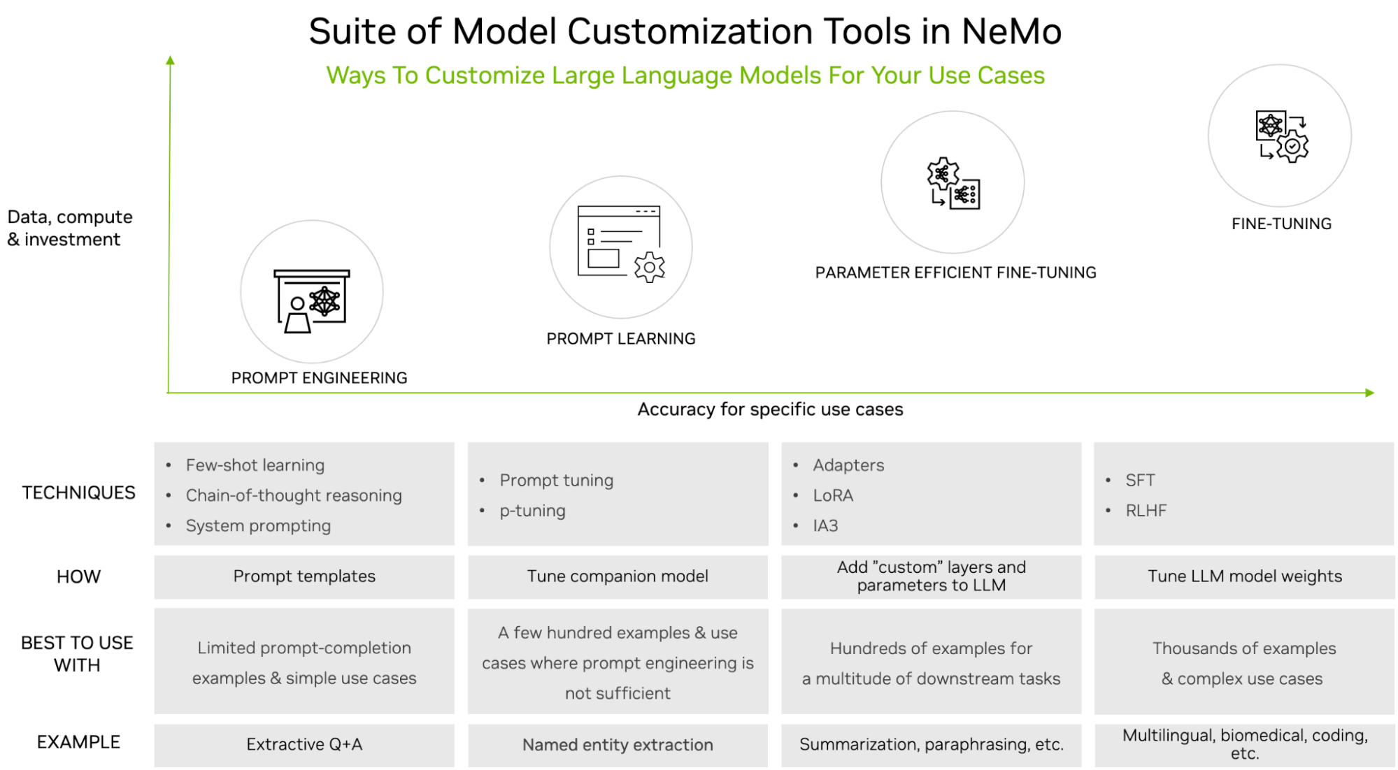
Figure 1 shows the following popular customization techniques:
- Prompt engineering: Manipulates the prompt sent to the LLM but doesn’t alter the parameters of the LLM in any way. It is light in terms of data and compute requirements.
- Prompt learning: Uses prompt and completion pairs imparting task-specific knowledge to LLMs through virtual tokens. This process requires more data and compute but provides better accuracy than prompt engineering.
- Parameter-efficient fine-tuning (PEFT): Introduces a small number of parameters or layers to existing LLM architecture and is trained with use-case–specific data, providing higher accuracy than prompt engineering and prompt learning, while requiring more training data and compute.
- Fine-tuning: Involves updating the pretrained LLM weights unlike the three types of customization techniques outlined earlier that keep these weights frozen. This means fine-tuning also requires the most amount of training data and compute as compared to these other techniques. However, it provides the most accuracy for specific use cases, justifying the cost and complexity.
For more information, see An Introduction to Large Language Models: Prompt Engineering and P-Tuning.
Prompt engineering
Prompt engineering involves customization at inference time with show-and-tell examples. An LLM is provided with example prompts and completions, detailed instructions that are prepended to a new prompt to generate the desired completion. The parameters of the model are not changed.
Few-shot prompting: This approach requires prepending a few sample prompts and completion pairs to the prompt, so that the LLM learns how to generate responses for a new unseen prompt. While few-shot prompting requires a relatively smaller amount of data as compared to other customization techniques and does not require fine-tuning, it does add to inference latency.
Chain-of-thought reasoning: Just as humans decompose bigger problems into smaller ones and apply chain of thought to solve problems effectively, chain-of-thought reasoning is a prompt engineering technique that helps LLMs improve their performance on multi-step tasks. It involves breaking a problem down into simpler steps with each of the steps requiring slow and deliberate reasoning. This approach works well for logical, arithmetic, and deductive reasoning tasks.
System prompting: This approach involves adding a system-level prompt in addition to the user prompt to provide specific and detailed instructions to the LLMs to behave as intended. The system prompt can be thought of as input to the LLM to generate its response. The quality and specificity of the system prompt can have a significant impact on the relevance and accuracy of the LLM’s response.
Prompt learning
Prompt learning is an efficient customization method that makes it possible to use pretrained LLMs on many downstream tasks without needing to tune the pretrained model’s full set of parameters. It includes two variations with subtle differences called p-tuning and prompt tuning; both methods are collectively referred to as prompt learning.
Prompt learning enables adding new tasks to LLMs without overwriting or disrupting previous tasks for which the model has already been pretrained. Because the original model parameters are frozen and never altered, prompt learning also avoids catastrophic forgetting issues often encountered when fine-tuning models. Catastrophic forgetting occurs when LLMs learn new behavior during the fine-tuning process at the cost of foundational knowledge gained during LLM pretraining.
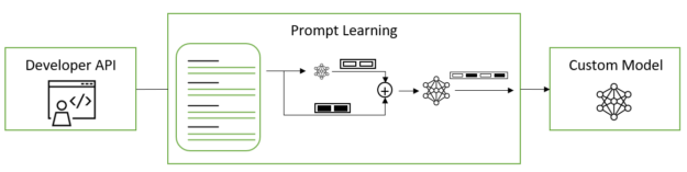
Instead of selecting discrete text prompts in a manual or automated fashion, prompt tuning and p-tuning use virtual prompt embeddings that you can optimize by gradient descent. These virtual token embeddings exist in contrast to the discrete, hard, or real tokens that do make up the model’s vocabulary. Virtual tokens are purely 1D vectors with dimensionality equal to that of each real token embedding. In training and inference, continuous token embeddings are inserted among discrete token embeddings according to a template provided in the model’s config.
Prompt tuning: For a pretrained LLM, soft prompt embeddings are initialized as a 2D matrix of size total_virtual_tokens Xhidden_size. Each task that the model is prompt-tuned to perform has its own associated 2D embedding matrix. Tasks do not share any parameters during training or inference. The NeMo framework prompt tuning implementation is based on The Power of Scale for Parameter-Efficient Prompt Tuning.
P-tuning: An LSTM or MLP model called prompt_encoder is used to predict virtual token embeddings. prompt_encoder parameters are randomly initialized at the start of p-tuning. All base LLM parameters are frozen, and only the prompt_encoder weights are updated at each training step. When p-tuning completes, prompt-tuned virtual tokens from prompt_encoder are automatically moved to prompt_table where all prompt-tuned and p-tuned soft prompts are stored. prompt_encoder is then removed from the model. This enables you to preserve previously p-tuned soft prompts while still maintaining the ability to add new p-tuned or prompt-tuned soft prompts in the future.
prompt_table uses the task name as a key to look up the correct virtual tokens for a specified task. The NeMo framework p-tuning implementation is based on GPT Understands, Too.
Parameter-efficient fine-tuning
Parameter-efficient fine-tuning (PEFT) techniques use clever optimizations to selectively add and update few parameters or layers to the original LLM architecture. Using PEFT, model parameters are trained for specific use cases. Pretrained LLM weights are kept frozen and significantly fewer parameters are updated during PEFT using domain and task-specific datasets. This enables LLMs to reach high accuracy on trained tasks.
There are several popular parameter-efficient alternatives to fine-tuning pretrained language models. Unlike prompt learning, these methods do not insert virtual prompts into the input. Instead, they introduce trainable layers into the transformer architecture for task-specific learning. This helps attain strong performance on downstream tasks while reducing the number of trainable parameters by several orders of magnitude (closer to 10,000x fewer parameters) compared to fine-tuning.
- Adapter Learning
- Infused Adapter by Inhibiting and Amplifying Inner Activations (IA3)
- Low-Rank Adaptation (LoRA)
Adapter Learning: Introduces small feed-forward layers in between the layers of the core transformer architecture. Only these layers (adapters) are trained at fine-tuning time for specific downstream tasks. The adapter layer generally uses a down-projection to project the input 

Adapter modules are usually initialized such that the initial output of the adapter is always zeros to prevent degradation of the original model’s performance due to the addition of such modules. The NeMo framework adapter implementation is based on Parameter-Efficient Transfer Learning for NLP.
IA3: Adds even fewer parameters, compared to adapters, which simply scale the hidden representations in the transformer layer using learned vectors. These scaling parameters can be trained for specific downstream tasks. The learned vectors lk, lv, and lff, respectively rescale the keys and values in attention mechanisms and the inner activations in position-wise feed-forward networks. This technique also makes mixed-task batches possible because each sequence of activations in the batch can be separately and cheaply multiplied by its associated learned task vector. The NeMo framework IA3 implementation is based on Few-Shot Parameter-Efficient Fine-Tuning is Better and Cheaper than In-Context Learning.
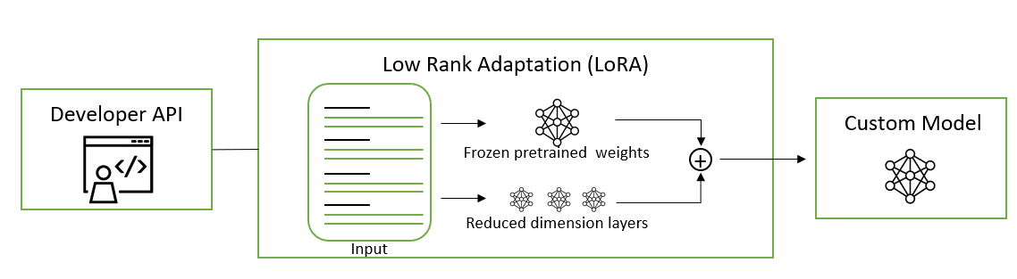
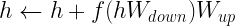
LoRA: Injects trainable low-rank matrices into transformer layers to approximate weight updates. Instead of updating the full pretrained weight matrix W, LoRA updates its low-rank decomposition, reducing the number of trainable parameters 10,000 times and the GPU memory requirements by 3x compared to fine-tuning. This update is applied to the query and value projection weight matrices in the multi-head attention sub-layer. Applying updates to low-rank decomposition instead of the entire matrix has been shown to be on par or better in model quality than fine-tuning, enabling higher training throughput and with no additional inference latency.
NeMo framework LoRA implementation is based on Low-Rank Adaptation of Large Language Models. For more information about how to apply the LoRa model to an extractive QA task, see the LoRA tutorial notebook.
Fine-tuning
When data and compute resources have no hard constraints, customization techniques such as supervised fine-tuning (SFT) and reinforcement learning with human feedback (RLHF) are great alternative approaches to PEFT and prompt engineering. Fine-tuning can help achieve the best accuracy on a range of use cases as compared to other customization approaches.
Supervised fine-tuning: SFT is the process of fine-tuning all the model’s parameters on labeled data of inputs and outputs that teaches the model domain-specific terms and how to follow user-specified instructions. It is typically done after model pretraining. Using pretrained models enables many benefits that include the use of state-of-the-art models without having to train from scratch, reduced computation costs, and reduced data collection needs as compared to the pretraining stage. A form of SFT is referred to as instruction tuning because it involves fine-tuning language models on a collection of datasets described through instructions.
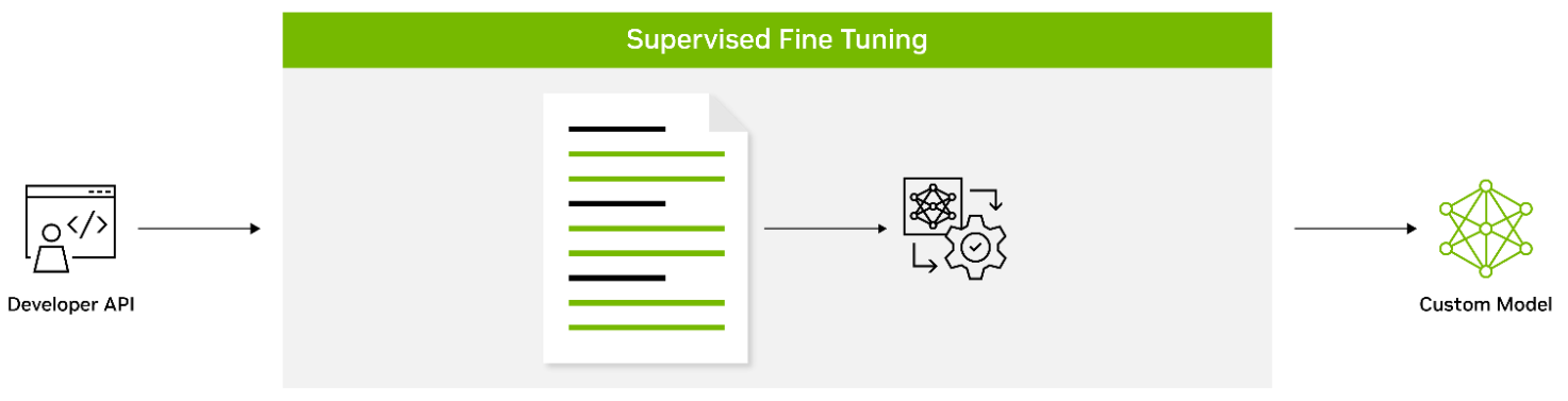
SFT with instructions leverages the intuition that NLP tasks can be described through natural language instructions, such as “Summarize the following article into three sentences.” or “Write an email in Spanish about an upcoming school festival.” This method successfully combines the strengths of fine-tuning and prompting paradigms to improve LLM zero-shot performance at inference time.
The instruction tuning process involves performing fine-tuning on the pretrained model on a mixture of several NLP datasets expressed through natural language instructions that are blended in varying proportions. At inference time, the fine-tuned model is evaluated on unseen tasks and this process is known to substantially improve zero-shot performance on unseen tasks. SFT is also an important intermediary step in the process of improving LLM capabilities using reinforcement learning, which we describe next.
Reinforcement learning with human feedback: Reinforcement learning with human feedback (RLHF) is a customization technique that enables LLMs to achieve better alignment with human values and preferences. It uses reinforcement learning to enable the model to adapt its behavior based on the feedback it receives. It involves a three-stage fine-tuning process that uses human preference as the loss function. The SFT model fine-tuned with instructions as described in the earlier section is considered the first stage in the RLHF technique.
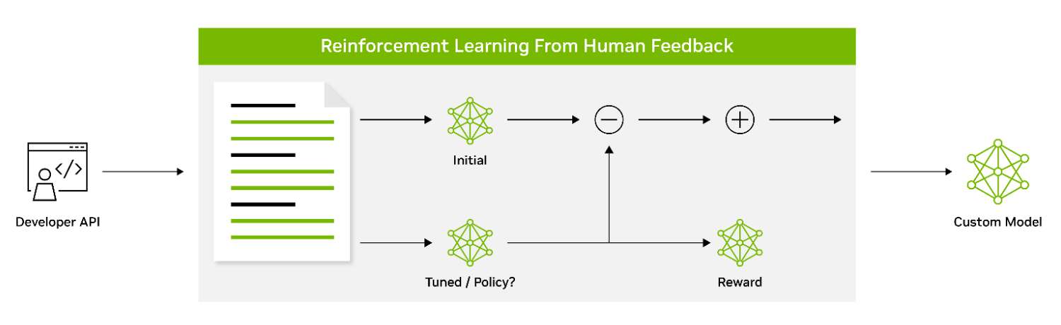
The SFT model is trained as a reward model (RM) in stage 2 of RLHF. A dataset consisting of prompts with multiple responses ranked by humans is used to train the RM to predict human preference.
After the RM is trained, stage 3 of RLHF focuses on fine-tuning the initial policy model against the RM using reinforcement learning with a proximal policy optimization (PPO) algorithm. These three stages of RLHF performed iteratively enable LLMs to generate outputs that are more aligned with human preferences and can follow instructions more effectively.
While RLHF results in powerful LLMs, the downside is that this method can be misused and exploited to generate undesirable or harmful content. The NeMo method uses the PPO value network as a critic model to guide the LLMs away from generating harmful content. There are other approaches being actively explored in the research community to steer the LLMs towards appropriate behavior and reduce toxic generation or hallucinations where LLMs make up facts.
Customize your LLMs
This post covered various model customization techniques and when to use them. Many of those methods are supported by NVIDIA NeMo.
NeMo provides an accelerated workflow for training with 3D parallelism techniques. It offers a choice of several customization techniques and is optimized for at-scale inference of large-scale models for language and image applications, with multi-GPU and multi-node configurations.
Download the NeMo framework today and customize pretrained LLMs on your preferred on-premises and cloud platforms.
 NVIDIA Modulus is now part of the NVIDIA AI Enterprise suite, supporting PyTorch 2.0, CUDA 12, and new samples.


 NVIDIA Nsight Developer Tools provide comprehensive access to NVIDIA GPUs and graphics APIs for performance analysis, optimization, and debugging activities….
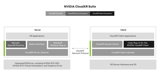
 NVIDIA is providing developers with an advanced platform to create scalable, branded, custom extended reality (XR) products with the new NVIDIA CloudXR Suite….