Categories
Offsites

Resolving High-Energy Impacts on Quantum Processors

Quantum processors are made of superconducting quantum bits (qubits) that — being quantum objects — are highly susceptible to even tiny amounts of environmental noise. This noise can cause errors in quantum computation that need to be addressed to continue advancing quantum computers. Our Sycamore processors are installed in specially designed cryostats, where they are sealed away from stray light and electromagnetic fields and are cooled down to very low temperatures to reduce thermal noise.

However, the world is full of high-energy radiation. In fact, there’s a tiny background of high-energy gamma rays and muons that pass through everything around us all the time. While these particles interact so weakly that they don’t cause any harm in our day-to-day lives, qubits are sensitive enough that even weak particle interactions can cause significant interference.

In “Resolving Catastrophic Error Bursts from Cosmic Rays in Large Arrays of Superconducting Qubits”, published in Nature Physics, we identify the effects of these high-energy particles when they impact the quantum processor. To detect and study individual impact events, we use new techniques in rapid, repetitive measurement to operate our processor like a particle detector. This allows us to characterize the resulting burst of errors as they spread through the chip, helping to better understand this important source of correlated errors.

The Dynamics of a High-Energy Impact
The Sycamore quantum processor is constructed with a very thin layer of superconducting aluminum on a silicon substrate, onto which a pattern is etched to define the qubits. At the center of each qubit is the Josephson junction, a superconducting component that defines the distinct energy levels of the qubit, which are used for computation. In a superconducting metal, electrons bind together into a macroscopic, quantum state, which allows electrons to flow as a current with zero resistance (a supercurrent). In superconducting qubits, information is encoded in different patterns of oscillating supercurrent going back and forth through the Josephson junction.

If enough energy is added to the system, the superconducting state can be broken up to produce quasiparticles. These quasiparticles are a problem, as they can absorb energy from the oscillating supercurrent and jump across the Josephson junction, which changes the qubit state and produces errors. To prevent any energy from being absorbed by the chip and producing quasiparticles, we use extensive shielding for electric and magnetic fields, and powerful cryogenic refrigerators to keep the chip near absolute zero temperature, thus minimizing the thermal energy.

A source of energy that we can’t effectively shield against is high-energy radiation, which includes charged particles and photons that can pass straight through most materials. One source of these particles are tiny amounts of radioactive elements that can be found everywhere, e.g., in building materials, the metal that makes up our cryostats, and even in the air. Another source is cosmic rays, which are extremely energetic particles produced by supernovae and black holes. When cosmic rays impact the upper atmosphere, they create a shower of high-energy particles that can travel all the way down to the surface and through our chip. Between radioactive impurities and cosmic ray showers, we expect a high energy particle to pass through a quantum chip every few seconds.

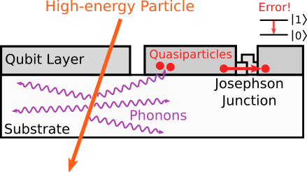
When a high-energy impact event occurs, energy spreads through the chip in the form of phonons. When these arrive at the superconducting qubit layer, they break up the superconducting state and produce quasiparticles, which cause the qubit errors we observe.

When one of these particles impinges on the chip, it passes straight through and deposits a small amount of its energy along its path through the substrate. Even a small amount of energy from these particles is a very large amount of energy for the qubits. Regardless of where the impact occurs, the energy quickly spreads throughout the entire chip through quantum vibrations called phonons. When these phonons hit the aluminum layer that makes up the qubits, they have more than enough energy to break the superconducting state and produce quasiparticles. So many quasiparticles are produced that the probability of the qubits interacting with one becomes very high. We see this as a sudden and significant increase in errors over the whole chip as those quasiparticles absorb energy from the qubits. Eventually, as phonons escape and the chip cools, these quasiparticles recombine back into the superconducting state, and the qubit error rates slowly return to normal.

A high-energy particle impact (at time = 0 ms) on a patch of the quantum processor, showing error rates for each qubit over time. The event starts by rapidly spreading error over the whole chip, before saturating and then slowly returning to equilibrium.

Detecting Particles with a Computer
The Sycamore processor is designed to perform quantum error correction (QEC) to improve the error rates and enable it to execute a variety of quantum algorithms. QEC provides an effective way of identifying and mitigating errors, provided they are sufficiently rare and independent. However, in the case of a high-energy particle going through the chip, all of the qubits will experience high error rates until the event cools off, producing a correlated error burst that QEC won’t be able to correct. In order to successfully perform QEC, we first have to understand what these impact events look like on the processor, which requires operating it like a particle detector.

To do so, we take advantage of recent advances in qubit state preparation and measurement to quickly prepare each qubit in their excited state, similar to flipping a classical bit from 0 to 1. We then wait for a short idle time and measure whether they are still excited. If the qubits are behaving normally, almost all of them will be. Further, the qubits that experience a decay out of their excited state won’t be correlated, meaning the qubits that have errors will be randomly distributed over the chip.

However, during the experiment we occasionally observe large error bursts, where all the qubits on the chip suddenly become more error prone all at once. This correlated error burst is a clear signature of a high-energy impact event. We also see that, while all qubits on the chip are affected by the event, the qubits with the highest error rates are all concentrated in a “hotspot” around the impact site, where slightly more energy is deposited into the qubit layer by the spreading phonons.

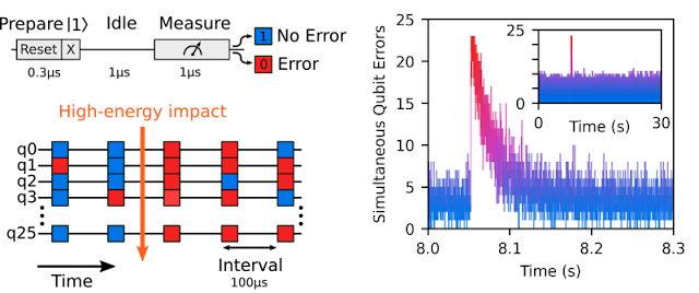
To detect high-energy impacts, we rapidly prepare the qubits in an excited state, wait a little time, and then check if they’ve maintained their state. An impact produces a correlated error burst, where all the qubits show a significantly elevated error rate, as shown around time = 8 seconds above.

Next Steps
Because these error bursts are severe and quickly cover the whole chip, they are a type of correlated error that QEC is unable to correct. Therefore, it’s very important to find a solution to mitigate these events in future processors that are expected to rely on QEC.

Shielding against these particles is very difficult and typically requires careful engineering and design of the cryostat and many meters of shielding, which becomes more impractical as processors grow in size. Another approach is to modify the chip, allowing it to tolerate impacts without causing widespread correlated errors. This is an approach taken in other complex superconducting devices like detectors for astronomical telescopes, where it’s not possible to use shielding. Examples of such mitigation strategies include adding additional metal layers to the chip to absorb phonons and prevent them from getting to the qubit, adding barriers in the chip to prevent phonons spreading over long distances, and adding traps for quasiparticles in the qubits themselves. By employing these techniques, future processors will be much more robust to these high-energy impact events.

As the error rates of quantum processors continue to decrease, and as we make progress in building a prototype of an error-corrected logical qubit, we’re increasingly pushed to study more exotic sources of error. While QEC is a powerful tool for correcting many kinds of errors, understanding and correcting more difficult sources of correlated errors will become increasingly important. We’re looking forward to future processor designs that can handle high energy impacts and enable the first experimental demonstrations of working quantum error correction.

Acknowledgements
This work wouldn’t have been possible without the contributions of the entire Google Quantum AI Team, especially those who worked to design, fabricate, install and calibrate the Sycamore processors used for this experiment. Special thanks to Rami Barends and Lev Ioffe, who led this project.

Categories
Misc

Hatch Me If You Can: Startup’s Sorting Machines Use AI to Protect Healthy Fish Eggs

Fisheries collect millions upon millions of fish eggs, protecting them from predators to increase fish yield and support the propagation of endangered species — but an issue with gathering so many eggs at once is that those infected with parasites can put healthy ones at risk. Jensorter, an Oregon-based startup, has created AI-powered fish egg Read article >

The post Hatch Me If You Can: Startup’s Sorting Machines Use AI to Protect Healthy Fish Eggs appeared first on The Official NVIDIA Blog.

Categories
Misc

EarlyStopping: ‘patience’ count is reset when tuning in Keras

I’m using keras-tuner to perform a hyperparameter optimization of a neural network.

I’m using a Hyperband optimization, and I call the search method as:

import keras_tuner as kt tuner = kt.Hyperband(ann_model, objective=Objective('val_loss', direction="min"), max_epochs=100, factor=2, directory=/path/to/folder, project_name="project_name", seed=0) tuner.search(training_gen(), epochs=50, validation_data=valid_gen(), callbacks=[stop_early], steps_per_epoch=1000, validation_freq=1, validation_steps=100) 

where the EarlyStopping callback is defined as:

stop_early = tf.keras.callbacks.EarlyStopping(monitor='val_loss', min_delta=0.1, mode='min', patience=15) 

Hyperband initially trains many models (each one with a different combination of the hyperparameters previously chosen) for only 2 epochs; then, it discards poor performing models and it only trains the most promising ones, step by step, with an increasing number of epochs at each step (the final goal is to discard all models except one, the best perfoming one).

So the training of a specific model is not performed in one shot, but it’s perfomed by steps, where in each of them Keras saves the state of the training.

By setting max_epochs=100, I noticed that the training of a model is performed by these steps (called “Runnning trials“):

  1. firstly, from epoch 1 to epoch 3;
  2. secondly, from 4 to 7;
  3. then, from 8 to 13;
  4. then, from 14 to 25;
  5. then, from 26 to 50;
  6. and finally, from 51 to 100.

So, at the end of each “Running trial”, Keras saves the state of the training, in order to continue, at the next “Running trial”, the training from that state.

By setting patience=15: during “Runnning trials” 1), 2), 3), 4) of the list above, EarlyStopping could not operate because the number of training epochs is less than patience; thus, EarlyStopping could operate only during “Running trials” 5) and 6) of the list above.

Initially I thought that the patience count started at epoch 1 and should never reset itself when a new “Running trial” begins, but I noticed that the EarlyStopping callback stops the training at epoch 41, thus during the “Running trial” 5), which goes from epoch 26 to 50 .
Thus it seems to me that, at the beginning of each “Running trial”, patience count is reset; indeed: EarlyStopping arrests the training at epoch 41, the first epoch at which EarlyStopping is able to operate, because: start_epoch + patience = 26 + 15 = 41..

Is it normal/expected behavior that patience is automatically reset at the beginning of each “Running trial” while using Keras Hyperband tuning?

submitted by /u/RainbowRedditForum
[visit reddit] [comments]

Categories
Misc

UK Biobank Advances Genomics Research with NVIDIA Clara Parabricks

UK Biobank is broadening scientists’ access to high-quality genomic data and analysis by making its massive dataset available in the cloud alongside NVIDIA GPU-accelerated analysis tools. Used by more than 25,000 registered researchers around the world, UK Biobank is a large-scale biomedical database and research resource with deidentified genetic datasets, along with medical imaging and Read article >

The post UK Biobank Advances Genomics Research with NVIDIA Clara Parabricks appeared first on The Official NVIDIA Blog.

Categories
Misc

A beginner question

tf.flags.DEFINE_string('config', '', 'Path to the file with configurations') 

What does this mean? What will be a better document to learn the basics of TF?

submitted by /u/Admirable-Study-626
[visit reddit] [comments]

Categories
Misc

Text prediction project – Finally managed to break the plateau by increasing the prob. of keeping weights. But I’m damn sure it will plateau again at some point, maybe the only thing could be changed at this point is the learning rate?

Text prediction project - Finally managed to break the plateau by increasing the prob. of keeping weights. But I'm damn sure it will plateau again at some point, maybe the only thing could be changed at this point is the learning rate? submitted by /u/Smsm1998
[visit reddit] [comments]
Categories
Misc

What returns on model.evaluate??

What returns on model.evaluate??

This may seem like a basic question but I am a little confused. In this example picture I call model.evaluate. The returned message says the batch_loss is 2.1455. But I had a callback keep track of the batch loss and if I calculate the mean of the batch_loss it is 2.0925, and 2.1455 is not seen in any of the callback loss values. So… What is evaluating returning here?

https://preview.redd.it/k2l2bt2pdzd81.png?width=536&format=png&auto=webp&s=7ec27ea483283e721c7053cdbf41ef0a22d3ff64

This is a custom model so it could be my implementation?? but it’s weird that it is so close but off.

Thanks!

submitted by /u/Dylan_TMB
[visit reddit] [comments]

Categories
Misc

Values of gradients to be returned

If I am making a function that has two inputs, what values is `tape.gradients` expecting?

For example, if I input data in a batch size to the function `f(x,y)`, the `tape.gradient` expects both of the returned gradients to be of shape (batch size, 2), however I’m not sure what should be the contents of those Tensors. For a batch size of 3, I thought it would look something like the following:

df/dx (x_1, y_1) df/dy (x_1, y_1)
df/dx (x_2, y_2) df/dy (x_2, y_2)
df/dx (x_3, y_3) df/dy (x_3, y_3)

Where the above table is a Tensor, but i have no idea what other tensor it could want for the second variable. Does anyone have an idea of what it should be? Thanks

submitted by /u/soravoid
[visit reddit] [comments]

Categories
Misc

NVIDIA Nsight Systems 2022.1 Introduces Vulkan 1.3 and Linux Backtrace Sampling and Profiling Improvements

The latest Nsight Systems 2022.1 release introduces several improvements aimed to enhance the profiling experience.

The latest update to NVIDIA Nsight Systems—a performance analysis tool designed to help developers tune and scale software across CPUs and GPUs—is now available for download. Nsight Systems 2022.1 introduces several improvements aimed to enhance the profiling experience. 

Nsight Systems is part of the powerful debugging and profiling NVIDIA Nsight Tools Suite. A developer can start with Nsight Systems for an overall system view and avoid picking less efficient optimizations based on assumptions and false-positive indicators. 

2022.1 highlights 

  • Vulkan 1.3 support.
  • System-wide CPU backtrace sampling and CPU context switch tracing on Linux.
  • NVIDIA NIC metrics sampling improvements.
  • MPI trace improvements.
  • Improvements for remote profiling over SSH. 

With Vulkan 1.3, you now have access to nearly two dozen new extensions. Some extensions, like VK_KHR_dynamic_rendering, help you to simplify your code while improving readability.

Other extensions, such as VK_KHR_shader_integer_dot_product or VK_EXT_pipeline_creation_cache_control, provide new functionality to help you build even better graphics applications. 

This release of Nsight Systems includes support for Vulkan 1.3 that helps you solve real world problems quickly and easily.

Figure 1. Vulkan 1.3 and ray tracing leadership video

The system-wide CPU thread context switch trace and backtrace sampling feature on Linux. Users will now be able to see if other apps, OS processes and kernel might be interfering with the processes you are profiling.

Workflow of backtrace sampling and CPU context switch tracing on Linux
Figure 2. System-wide CPU backtrace sampling and CPU context switch tracing on Linux.

More information 

Categories
Misc

Overcoming Data Collection and Augmentation Roadblocks with NVIDIA TAO Toolkit and Appen Data Annotation Platform

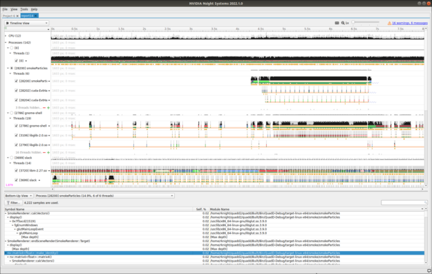
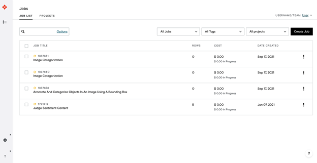
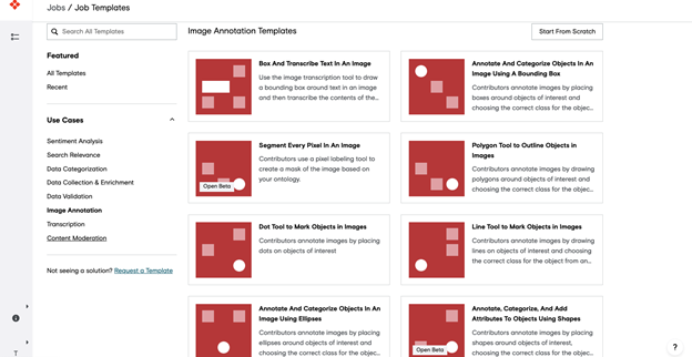
Generating and labeling data to train AI models is time-consuming. Appen, helps label and annotate your data, which can then be used as inputs in the TAO Toolkit.
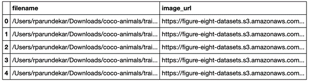
Building AI models from scratch requires enormous amounts of data, time, money, and expertise. This is at odds with what it takes to succeed in the AI space: fast time-to-market and the ability to quickly evolve and customize solutions. NVIDIA TAO, an AI-Model-Adaptation framework, enables you to leverage production-quality, pretrained AI models and fine-tune them in a fraction of the time compared to training from scratch.

To fine-tune these models further, or confirm the precision of your model, additional high-quality training data is required. Appen, a data annotation partner for TAO, provides access to high-quality datasets and services to label and annotate your data for your unique needs, if you don’t have the right data available.

In the post, I show you how you can use the NVIDIA TAO Toolkit, a CLI-based solution of the NVIDIA TAO framework, along with Appen’s data labeling platform to simplify the overall training process and create highly customized models for a particular use case.

After your team has identified a business problem to solve using ML, you can select from NVIDIA collection of pretrained AI models in computer vision and conversational AI. Computer vision models can include face detection models, text recognition, segmentation, and more. Then you can apply the TAO Toolkit to build, train, test, and deploy your solution.

To speed up the data collection and augmentation process, you can now use the Appen Data Annotation Platform to create the right training data for your use case. The robust platform enables you to access Appen’s global crowd of over one million skilled annotators from over 170 countries, speaking 235 languages. Appen’s data annotation platform and expertise also provide you with other resources:

  • High-quality datasets (for when you need data)
  • Human labelers sourced globally to annotate your unlabeled data
  • An easy-to-use platform where you can launch annotation jobs and monitor key metrics
  • Quality assurance checks and data security controls

With clean, high-quality data, you can adapt pretrained NVIDIA models to suit your requirements, pruning, and retraining to achieve the performance level that you need.

How to prepare your data using Appen’s platform

If you don’t already have data to use for training your model, you can either collect that data yourself or turn to Appen to source datasets that suit your use cases. The Appen Data Annotation Platform (ADAP) works with a diverse set of formats:

  • Audio (.wav, .mp3)
  • Image (.jpeg, .png)
  • Text (.txt)
  • Video (URL)

When you’re done with the data collection phase, unless you plan to work with Appen for your data collection needs, you can use Appen’s platform to quickly label the data you’ve collected. You need an Appen platform license and budget for each row of data annotation.

From there, work through the following steps to deploy a model that works specifically for your needs. For the purposes of this post, assume that you’re annotating images for an object detection model.

Prepare your data

First, load your image data into a web-accessible location: the cloud or a location that ADAP can access, such as a private Amazon S3 bucket.

Next, structure your input CSV file with two columns. The first column contains the filenames, and the second includes URLs to the images. You can provide the URLs in one of three ways:

  • Use publicly available URLs for your data.
  • Use presigned URLs.
  • Use Appen’s Secure Data Access tool, which you can use to attach your database securely to the platform; Appen only accesses your data when needed.

The second column contains the local file name on your device. Figure 1 shows what your CSV file may look like.

Three columns of data (labels, filename, and image_url), five rows labeled 0 to 4 with names and URLs.
Figure 1. CSV structure for data upload in ADAP

Create your job and upload data

If you haven’t already, you can create an ADAP account and sign in. You must have an active license for the platform before running new jobs. To learn more about plans and pricing, contact Appen.

After logging in, under Jobs, choose Create a Job.

A window with four job rows, job titles, ids, rows, cost, date created. In the header, there is a search box and three filters, as well as the Create Job button.
Figure 2. ADAP jobs overview page

Select the template that best fits the job (sentiment analysis, search relevance, and so on). For this example, choose Image Annotation.

Prebuilt annotation job templates sorted by use case, with filters and search. Current view is filtered on Image annotation templates. There is a start from scratch button available.
Figure 3. ADAP job templates page – Image annotation

Under Image Annotation, choose Annotate and Categorize Objects in an Image Using a Bounding Box. Upload your CSV file by dragging and dropping it into the Upload tab.

Design your job

Provide guidelines for Appen’s crowd of over one million data labelers on what they should be looking for and any requirements that they should be aware of. The template provides a simple job design to help you get started.

Next, choose Manage the Image Annotation Ontology, where you’ll define the classes that should be detected. Update the instructions to give more context about your use case and describe how annotators should identify and label objects in images. You can preview your job and see how an annotator will view it.

Finally, create test questions to measure and track labeler performance.

Launch job

Do a test run first before officially launching your annotation job on the platform. After you’ve launched your job, Appen’s global crowd of data labelers annotate your data to your specifications.

Monitor

Monitor the accuracy rate of annotations in real time. Adjust as needed in areas like job design, test questions, or annotators.

A page that analyzes annotation job progress by displaying charts about completion rate, rows finalized, pending judgements, total costs and rows uploaded.
Figure 8. ADAP annotation progress monitoring page

Results

Download a report of your labeled data output by choosing Download, Full.

Convert output to KITTI format

From here, you need a script to convert your labeled data to a format that’s feedable to the TAO Toolkit, such as KITTI format.

Using the output from the previous step, you can use the following section to convert your labeled data to a format like the Pascal Visual Object Classes (VOC) format. For the full code and guide on how to convert your data, see the /Appen/public-demos GitHub repo.

Training your model

Your data annotated with Appen can now be used to train your object detection model. The TAO Toolkit allows you to train, fine-tune, prune, and export highly optimized and accurate AI models for deployment by adapting popular network architectures and backbones to your data. For this example, you can choose a YOLOV3 Object Detection model, as in the following example:

First, download the notebook.

$ wget --content-disposition https://api.ngc.nvidia.com/v2/resources/nvidia/tlt_cv_samples/versions/v1.0.2/zip -O tlt_cv_samples_v1.0.2.zip

$ unzip -u tlt_cv_samples_v1.0.2.zip  -d ./tlt_cv_samples_v1.0.2 && rm -rf tlt_cv_samples_v1.0.2.zip && cd ./tlt_cv_samples_v1.0.2

After the notebook samples are downloaded, you may start the notebook using the following commands:

$ jupyter notebook --ip 0.0.0.0 --port 8888 --allow-root

Open the internet browser on localhost and open the following URL:

http://0.0.0.0:8888

Because you are creating a YOLOv3 model, open the yolo_v3/yolo_v3.ipynb notebook. Follow the notebook instructions to train the model.

Based on results, fine-tune the model until it achieves your metric goals. If desired, you can create your own active learning loop at this stage. Prioritize data based on confidence or another selection metric using the CSV file method as described in the preceding steps. You can also load data (including inputs and predictions) beforehand so Appen’s annotators can validate the model after it’s been trained, reviewing the predictions using our domain experts and open crowd.

Pro tip: Use Workflows, an Appen Solution, to build and automate multistep data annotation projects with ease.

Iterate

Appen can further assist you with data collection and annotation in subsequent rounds of model training as you iteratively improve on your model performance. To avoid model drift or to accommodate changing business requirements, retrain your model regularly.

Conclusion

NVIDIA TAO Toolkit combined with Appen’s data platform enables you to train, fine-tune, and optimize pretrained models to get your AI solutions off the ground faster. Speed up your development times by tenfold without sacrificing quality. With the help of integrated expertise and tools from NVIDIA and Appen, you’ll be ready to launch AI with confidence.

For more information, see the following resources: