Categories
Misc

Validating NVIDIA DRIVE Sim Camera Models

A view from a camera model rendered in NVIDIA DRIVE Sim.This post covers the validation of camera models in DRIVE Sim, assessing the performance elements, from rendering of the world scene to protocol simulation.A view from a camera model rendered in NVIDIA DRIVE Sim.

Autonomous vehicles require large-scale development and testing in a wide range of scenarios before they can be deployed.

Simulation can address these challenges by delivering scalable, repeatable environments for autonomous vehicles to encounter the rare and dangerous scenarios necessary for training, testing, and validation.

NVIDIA DRIVE Sim on Omniverse is a simulation platform purpose-built for development and testing of autonomous vehicles (AV). It provides a high-fidelity digital twin of the vehicle, the 3D environment, and the sensors needed for the development and validation of AV systems.

Unlike virtual worlds for other applications such as video games, DRIVE Sim must generate data that accurately models the real-world. Using simulation in an engineering toolchain requires a clear grasp of the simulator’s performance and limitations. 

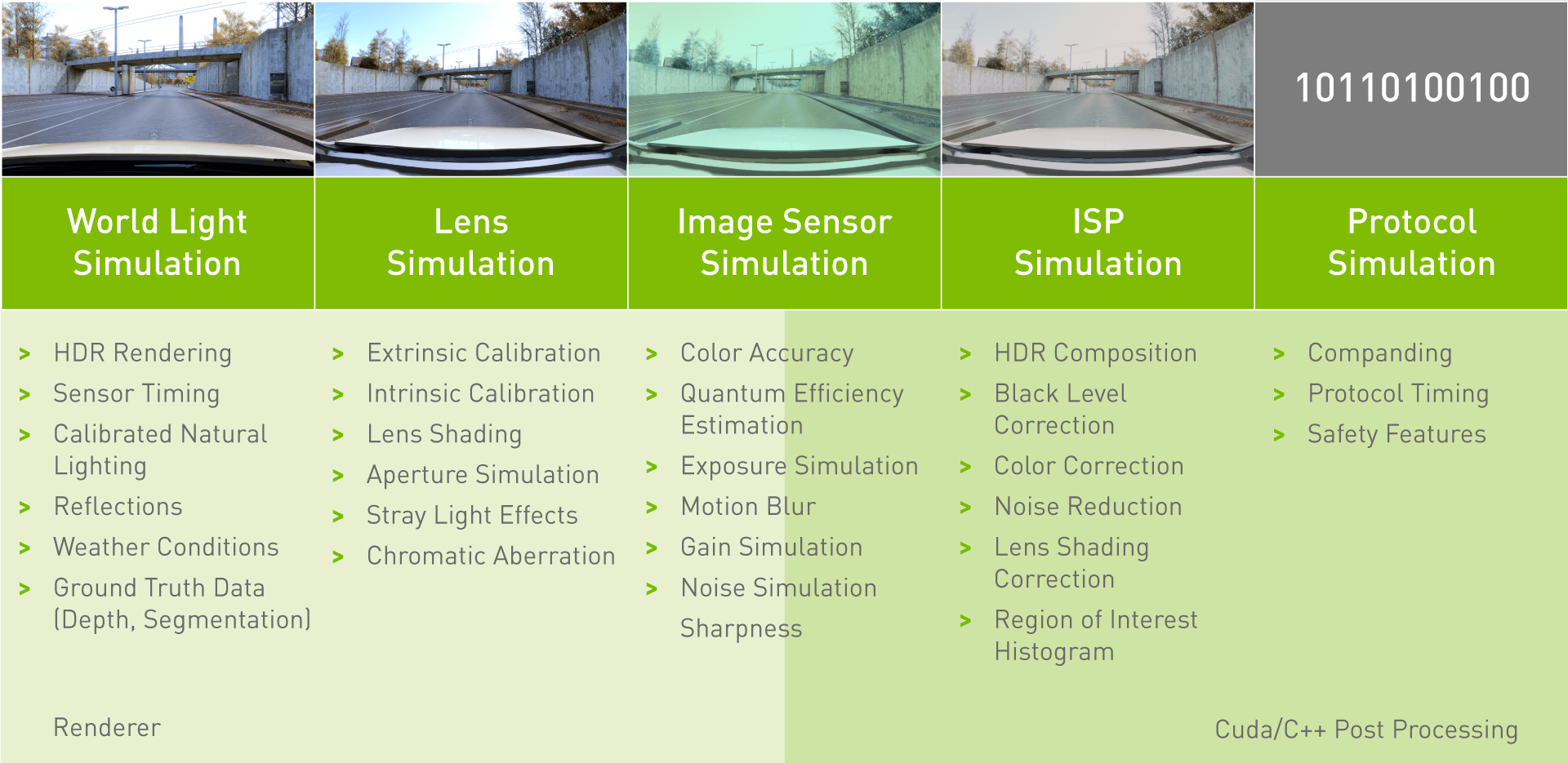
This accuracy covers all of the functions modeled by the simulator including vehicle dynamics, vehicle components, behavior of other drivers and pedestrians, and the vehicle’s sensors. This post covers part of the validation of camera models in DRIVE Sim, which requires assessing the individual performance of each element, from rendering of the world scene to protocol simulation. 

Validating a camera simulation model

A thorough validation of a simulated camera can be performed with two methodologies:

  • Individual analysis of each component of the model ( Figure 1).
  • A top-down verification that the camera data produced by a simulator accurately represents the real camera data in practice, for instance, by comparing the performance of perception models trained on real or synthetic images.

Individual component analysis is a complex topic. This post describes our component-level validation of two critical properties of the camera model: camera calibration (extrinsic and intrinsic parameters) and color accuracy. Direct comparisons are made with real world camera data to identify any delta between simulated and real world images. 

A table summarizing the components of an autonomous vehicle camera model.
Figure 1.  Summary of camera model components

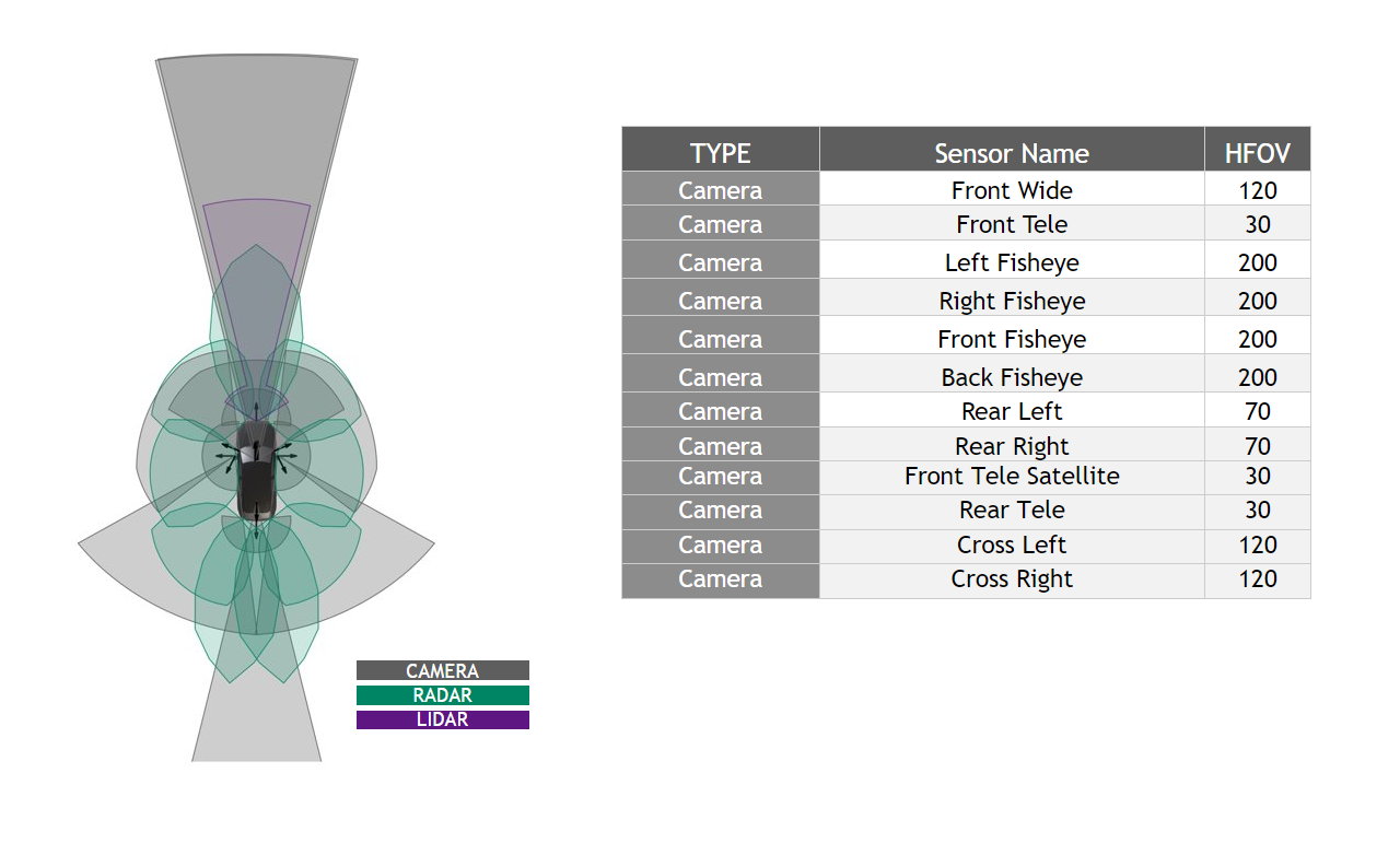
For this validation, we chose to use a set of camera models from the NVIDIA DRIVE Hyperion sensor suite. Figure 2 details the camera models used throughout testing. 

A breakdown of the NVIDIA DRIVE Hyperion 8 sensor set.
Figure 2.  NVIDIA DRIVE Hyperion 8 sensor set

Camera calibration

AV perception requires a precise understanding of where the cameras are positioned on the vehicle and how each unique lens geometry of a camera affects the images it produces. The AV system processes these parameters through camera calibration. 

A simulated camera sensor should accurately reproduce the images of a real camera when subjected to the same calibration and a digital twin environment. Likewise, simulated camera images should be able to produce similar calibration parameters as their real counterparts when fed into a calibration tool. 

We use NVIDIA Driveworks, our sensor calibration interface, to estimate all camera parameters mentioned in this post. 

Validation of camera characteristics can be done in these steps:

  • Extrinsic validation: Camera extrinsics are the characteristics of a camera sensor that describe its position and orientation on the vehicle. The purpose of extrinsic validation is to ensure that the simulator can accurately reproduce an image from a real sensor at a given position and orientation.
  • Calibration validation: The accuracy of the calibration is verified by computing the reprojection error. In real-world calibrations, this approach is used to quantify whether the calibration was valid and successful. We apply this step here to calculate the distance between key detected features reprojected on real and simulated images.

Intrinsic validation

Intrinsic camera calibration describes the unique geometry of an individual lens more precisely than its manufacturing tolerance by setting coefficients of a polynomial.

theta=c0+c1r+c2r^2 +c3r^3+c4r^4

  • r is the distance in pixels to the distortion center
  • c0,c1,c2,c3,c4 are the coefficients of the distortion function
  • theta (theta) is the resulting projection angle in radians

The calibration of this polynomial enables an AV to make better inferences from camera data by characterizing the effects of lens distortion. The difference between two lens models can be quantified by calculating the max theta distortion between them.

Diagram showing the maximum theta distortion.
Figure 3.  Max theta distortion diagram

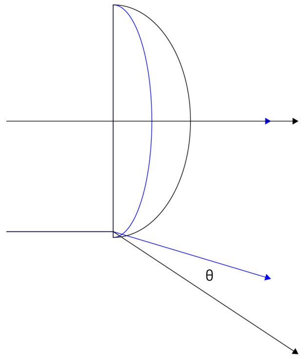
Max theta distortion describes the angular difference of light passing through the edge of a lens (corresponding to the edge of an image), where distortion is maximized. In this test, we will use the max theta distortion to describe the difference between a lens model generated from real calibration images and one from synthetic images.

We validate the intrinsic calibration of our simulated cameras according to the following process:

Figure 4. Intrinsic validation process
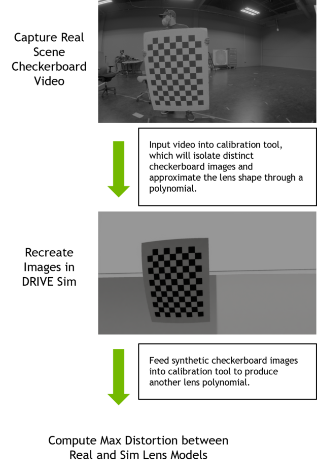
  1. Perform intrinsic camera calibration: Mounted cameras on a vehicle or test stand capture video of a checkerboard chart moving through each camera’s field of view at varying distances and degrees of tilt. This video is input into the DriveWorks Intrinsics Constraints Tool, which will pull distinct checkerboard images from it and output the polynomial coefficients for each camera in the calibration.
  2. Produce simulated checkerboard calibration images: The real camera lens calibration data are used to recreate each camera in DRIVE Sim. We recreate the real checkerboard images in simulation from the estimated chart positions and orientations output by the calibration tools.
  3. Produce intrinsic calibration from synthetic images: We input synthetic images into DriveWorks calibration tools to produce new polynomial coefficients.
  4. Compute max theta distortion from real to simulated lens: For each lens, we compare the geometry defined by the calibration from real images to the geometry defined by the calibration from the simulated images. We then find the point where the angle that light passes through varies most between the two lenses. The variation is reported as a percentage of the theoretical field of view of that lens (/(FOV*100)).

The max theta distortion for each camera derived by comparing its real f-theta lens calibration to the calibration yielded from simulated images.

Chart comparing the maximum theta distortion from the F-theta model.
Figure 5.  Max theta distortion from F-theta model

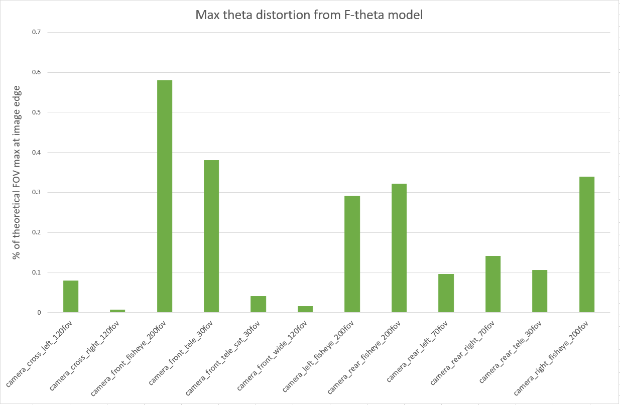
This first result exceeded our expectations as the simulation is behaving predictably and reproducing the observed outcomes from real-world calibrations.

This comparison provides a first degree of confidence in the ability of our model to accurately represent lens distortion effects because we observe a small discrepancy between real and simulated cameras. The front telephoto lens is difficult to constrain in real life, hence we expected it to be an outlier in our simulation results.

The fisheye cameras calibrations exhibit the largest real-to-sim difference (0.58% of FOV for the front fisheye camera).

Another way to look at these results is by considering the effect of the distortions on the generated images. We compare the real and simulated detected features from the calibration charts in a later step, described under the Numerical Feature Marker comparison.

We proceed with the extrinsic validation method.

Extrinsic validation

We validate the extrinsic calibration of our simulated cameras according to the following process:

  1. Perform extrinsic camera calibration: Mounted cameras on a vehicle or test stand capture images of multiple calibration patterns (AprilTag charts) located throughout the lab. For our test, cameras were mounted per the NVIDIA DRIVE Hyperion Level 2+ reference architecture.  Using the DriveWorks calibration tool, we calculate the exact position and orientation of the camera and the calibration charts in 3D space.
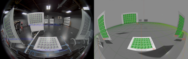
  2. Recreate scene in simulation: Using extrinsic parameters from real calibration and ground truth of AprilTag chart locations, the cameras and charts are spawned in simulation at the same relative positions and orientations as in the real lab. The system generates synthetic images from each of the simulated cameras.
  3. Produce extrinsic calibration from synthetic images and compare to real calibration: Synthetic images are inputted into DriveWorks calibration tools to output the position and orientation of all cameras and charts in the scene. We calculate the 3D differences between extrinsic parameters derived from real vs. synthetic calibration images.
A diagram of the extrinsic validation process.
Figure 6.  Extrinsic validation process

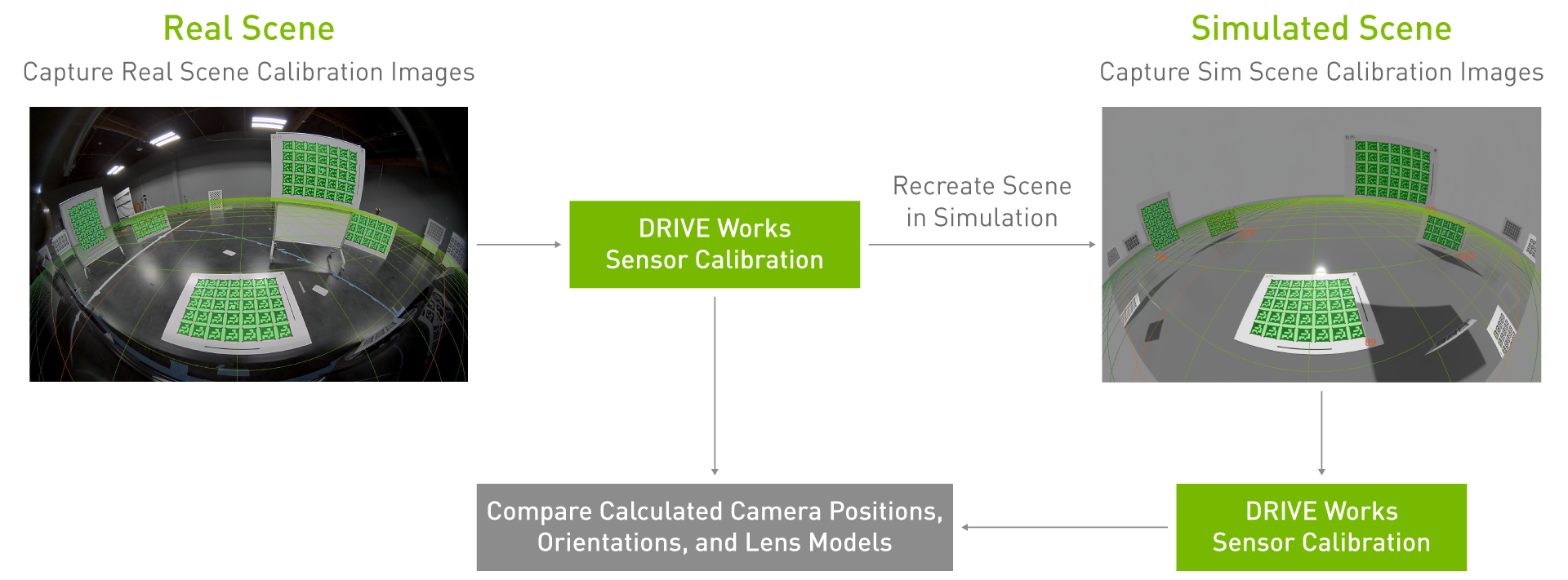
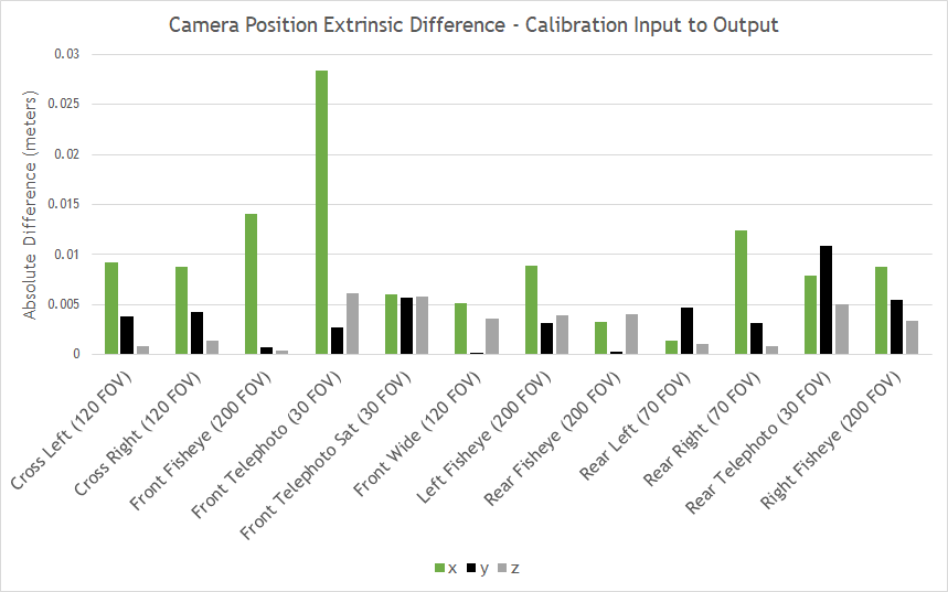
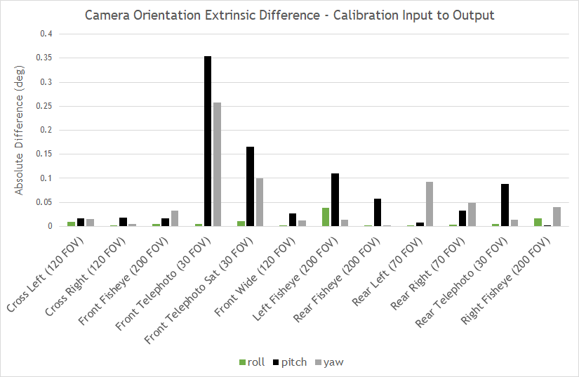
Figure 7 shows the differences in extrinsic parameters for each of the 12 cameras on the tested camera rig, comparing the real camera calibration to the calibration yielded by the simulated camera images. All camera position parameters matched within 3 cm and all camera orientation parameters matched within 0.4 degrees.

All positions and orientations are given with regard to a right-handed reference coordinate system with origin at the center of the rear axle of the car projected onto the ground plane, where x aligns with the direction of the car, y to the left, and z up. Yaw, pitch, and roll are counter-clockwise rotations around z, y, and x.

Graph comparing the camera position extrinsic differences, calibration input to output.
Figure 7.  Camera position extrinsic differences–calibration input to output
Graph comparing the camera orientation extrinsic differences, from calibration input to output.
Figure 8.  Camera orientation extrinsic differences–calibration input to output

Results

The validation previously described compares real lab calibrations to digital twins’ calibrations in DRIVE Sim RTX renderer. The RTX renderer is a path-tracing renderer that provides two rendering modes, a real-time mode and a reference mode (not real-time, focus on accuracy) to provide full flexibility depending on the specific use case.

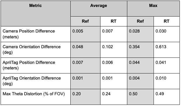
This full validation process was done with digital twins rendered in both RTX real-time and reference modes to evaluate the effect of reduced processing power allocated to rendering. See a summary of the real-time validation results in the following table, with reference results available for comparison.

As expected, there was a slight increase in real-to-sim error for most measurements when rendering in real-time due to reduced image quality. Nonetheless, calibration based on real-time images matched lab calibrations within 0.030 meters and 0.041 degrees for cameras, 0.041 meters and 0.010 degrees for AprilTag locations, and 0.49% of theoretical field of view for the lens models.

Table comparing reference to real-time validation results.
Figure 9.  Reference vs. real-time validation results

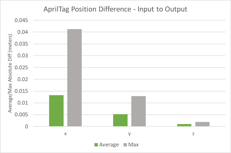
The following figures indicate the average and max position or orientation differences across 22 AprilTag charts located in the real and simulated environments. The average position difference from the real charts to their digital twins was less than 1.5 cm along all axes and no individual chart’s position difference exceeded 4.5 cm along any axis.

The average orientation difference from the real charts to their digital twins was less than 0.001 degrees for all axes and no individual chart’s orientation difference exceeded 0.004 degrees along any axis.

Graph comparing the average and maximum AprilTag orientation differences.
Figure 10. Average/max AprilTag orientation differences–calibration input to output

There is currently no standard to define an acceptable error under which a sensor simulation model can be deemed viable. Thus, we compare our position and orientation delta values to the calibration error yielded by real-world calibrations to define a valid criterion for the maximum acceptable error for our simulation. The resulting errors from our tests are consistently smaller than the calibration error observed in the real world.

This calibration method is based on statistical optimization techniques used by our calibration tool and hence can introduce its own uncertainty.  However, it is also important to note that the DriveWorks calibration system has been consistently used in research and development for sensor calibration with a high degree of accuracy.

These results also demonstrate that the calibration tool can function with simulation-rendered images and provide comparable results with the real world. The fact that the real-world calibration system and our simulation are in agreement is a first significant indicator of confidence for our camera simulation model.

Moreover, this method also validates the simulator as a whole, because the digital twin used for calibration models the scene in its entirety with all 12 cameras, without tweaking values to improve results.

To assess further the validity of this method, we then run a direct numerical feature marker comparison between the real and simulated images.

Numerical feature markers comparison

The calibration tool provides a visual validator to reproject the calibration charts positions onto the input images based on the estimated intrinsic parameters. The images show an example of the overlay of the detected features and the reprojection statistics (mean, std, min, and max reprojection error) for the simulated and real camera.

Image showing the overlay target positions onto input images.
Figure 11. Overlay target positions onto input images for camera_rear_fisheye_200fov

Computing the reprojection error enables us to assert further the validity of the prior calibration method. This approach parses the calibration tool’s detected features and compares them to the ones in the real image.

Here we consider the corners of each of the AprilTags in the calibration charts as the feature markers. We calculate the distance in pixels between the feature markers detected on real images compared to synthetic images, both for path-traced and real-time simulation.

The following figure shows an average distance of 1.4 pixels between reference path-traced simulated and real feature markers. The same comparison based on the real-time simulated dataset yields an average reprojection error of 1.62 pixels.

Graph comparing the average reprojection error of each camera model.
Figure 12.  Average reprojection error (reference vs. real time)

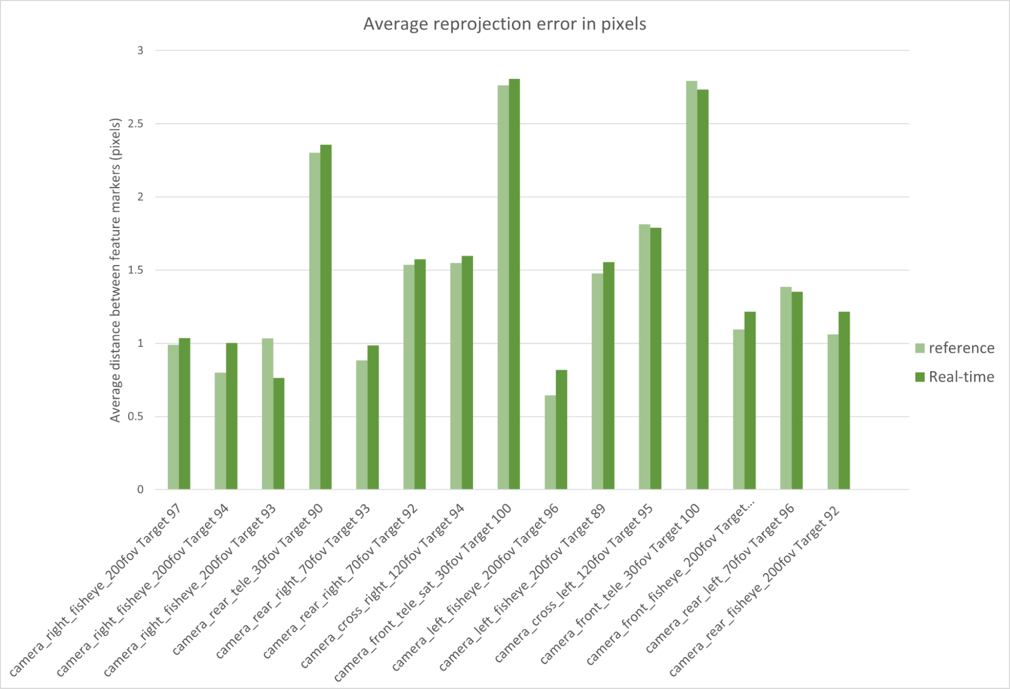
Both values are the real-world projection error threshold of 2 pixels used to evaluate the accuracy of the real-world calibrations. The results are very promising, in particular because this method is less dependent on the inner workings of our calibration tool.

In fact, the calibration tool is only used here to estimate the detected feature markers in each image. The comparison of the markers is done based on a purely algorithmic analysis of objects in 3D space.

Color accuracy assessment

The camera calibration results demonstrate pixel correspondence of images produced by our camera sensor model to their real image counterparts. The next step is to validate that the values associated with each of those pixels are accurate.

We simulated a Macbeth ColorChecker chart and captured an image of it in DRIVE Sim to validate image quality. The RGB values of each color patch were then compared to those of the corresponding real image.

In addition to the real images, we also introduced the Iray renderer, NVIDIA’s most realistic physical light simulator, validated against CIE 171:2006. We performed this test first using simulated images generated with the Iray rendering system, then with NVIDIA RTX renderer. The comparison with Iray gives a good measure of the capability of the RTX renderer against a recognized industry gold standard.

Sketch depicting the image quality test setup.
Figure 13. Image quality test setup

We validate the image quality of our simulated cameras according to the following process:

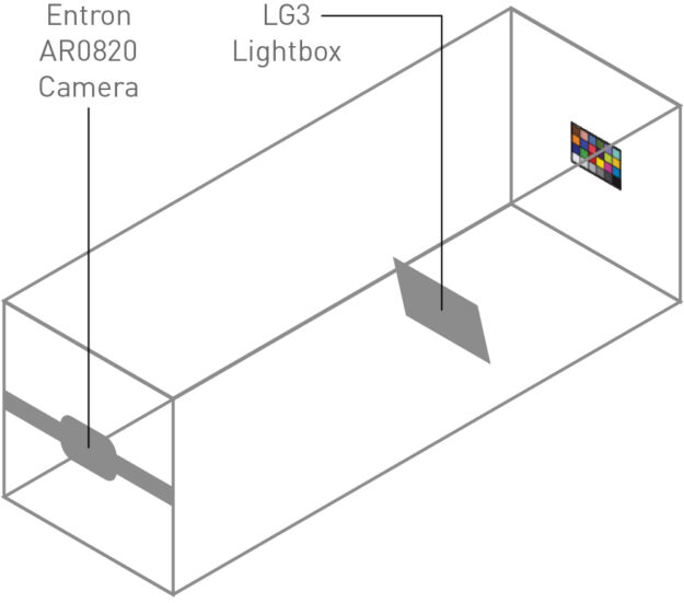
  1. Capture image of Macbeth ColorChecker chart in test chamber: A Macbeth ColorChecker chart is placed at a measured height and illuminated with a characterized external light source. The camera is placed at a known height and distance from the Macbeth chart.
  2. Re-create image in simulation: Using the dimensions of the test setup, calibrated Macbeth chart values, and the external lighting profile, we render the test scene using the DRIVE Sim RTX renderer. We then use our predefined camera model to recreate the images captured in the lab.
  3. Extract mean brightness and RGB values for each patch: We average the color values across all pixels in each patch for all three images (real, Iray, DRIVE Sim RTX renderer).
  4. Compare white-balanced brightness and RGB values: Measurements are normalized for each patch against patch 19 for white-balancing. We compare the balanced color and brightness values across the real image, Iray rendering, and RTX rendering.
A diagram of the MacBeth ColorChecker test process.
Figure 14.  Macbeth ColorChecker test process
An image of the Macbeth ColorChecker reference chart.
Figure 15.  Macbeth ColorChecker reference chart
Chart comparing real and rendered luma and RGB.
Figure 16.  Real and rendered luma and RGB comparisons
Chart comparing red color contributions of rendered images to real images.
Figure 17.  Comparison of red color contributions, rendered images vs real image
Chart comparing green color contributions of rendered images to real images.
Figure 18. Comparison of green color contributions, rendered images vs real image
Chart comparing blue color contributions of rendered images to real images.
Figure 19.  Comparison of blue color contributions, rendered images vs real image

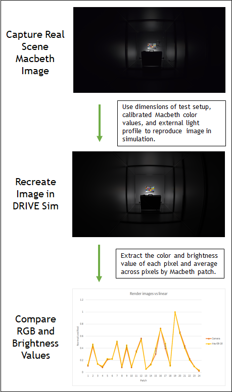
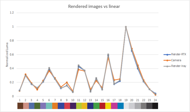
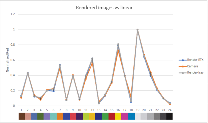
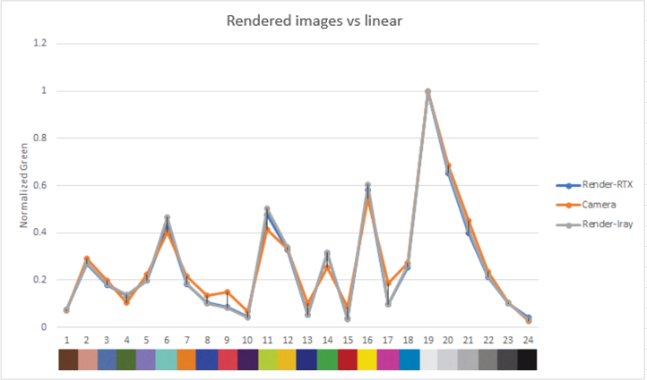
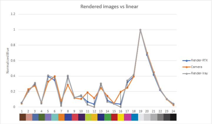
The graphs show the normalized luma and RGB output for each color patch in the rendered and real images.

Both the luma and RGB values for our rendered images are close to the real camera, which gives confidence in the ability of our sensor model to reproduce color and brightness contributions accurately.

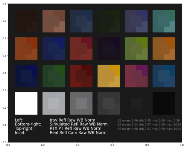
For a direct visual comparison, we show the stitched white-balanced RGB values of the Macbeth chart real and synthetic images (Iray, real-time, and path-traced contributions).

Figure 20. Stitched RGB patches Macbeth color chart (synthetic vs. real)

We also compute ΔE (see results in Figure 22), a CIE2000 computer vision metric, which quantifies the distance between the rendered and original camera values and is often used for camera characterization. A lower ΔE value indicates greater color accuracy and the human eye cannot detect a value under 1.

Table comparing CIE2000 sensor reference to real-time results.
Figure 21. Reference vs. real-time results for CIE2000

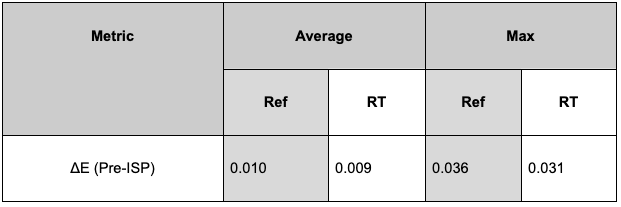
While ΔE provides a good measure of perceptual color difference and is recognized as an imaging standard, it is limited to human perception. The impact of such a metric on a neural network will remain to be evaluated in further tests.

Conclusion

This post presented the NVIDIA validation approach and preliminary results for our DRIVE Sim camera sensor model.

  • We conclude that our model can accurately reproduce real cameras’ calibrations parameters with an overall error that is below real-world calibration error.
  • We also quantified the color accuracy of our model with reference to the industry standard Macbeth color checker and found that it is closely aligned with typical R&D error margins.
  • In addition, we conclude that RTX real time rendering is a viable tool to achieve this level of accuracy.

This confirms that the DRIVE Sim camera model can reproduce the previously mentioned parameters of a real-world camera in a simulated environment at least as accurately as a twin camera setup in the real world. More importantly, these tests provide confidence to users that the outputs of the camera models, as far as intrinsics, extrinsics, and color reproduction, will be accurate and can serve as a foundation for other validation work to come.

The next steps will be to validate our model in the context of its real-world perception use cases and provide further results on imaging KPIs for the model in open-loop.

Categories
Offsites

A Scalable Approach for Partially Local Federated Learning

Federated learning enables users to train a model without sending raw data to a central server, thus avoiding the collection of privacy-sensitive data. Often this is done by learning a single global model for all users, even though the users may differ in their data distributions. For example, users of a mobile keyboard application may collaborate to train a suggestion model but have different preferences for the suggestions. This heterogeneity has motivated algorithms that can personalize a global model for each user.

However, in some settings privacy considerations may prohibit learning a fully global model. Consider models with user-specific embeddings, such as matrix factorization models for recommender systems. Training a fully global federated model would involve sending user embedding updates to a central server, which could potentially reveal the preferences encoded in the embeddings. Even for models without user-specific embeddings, having some parameters be completely local to user devices would reduce server-client communication and responsibly personalize those parameters to each user.

Left: A matrix factorization model with a user matrix P and items matrix Q. The user embedding for a user u (Pu) and item embedding for item i (Qi) are trained to predict the user’s rating for that item (Rui). Right: Applying federated learning approaches to learn a global model can involve sending updates for Pu to a central server, potentially leaking individual user preferences.

In “Federated Reconstruction: Partially Local Federated Learning”, presented at NeurIPS 2021, we introduce an approach that enables scalable partially local federated learning, where some model parameters are never aggregated on the server. For matrix factorization, this approach trains a recommender model while keeping user embeddings local to each user device. For other models, this approach trains a portion of the model to be completely personal for each user while avoiding communication of these parameters. We successfully deployed partially local federated learning to Gboard, resulting in better recommendations for hundreds of millions of keyboard users. We’re also releasing a TensorFlow Federated tutorial demonstrating how to use Federated Reconstruction.

Federated Reconstruction
Previous approaches for partially local federated learning used stateful algorithms, which require user devices to store a state across rounds of federated training. Specifically, these approaches required devices to store local parameters across rounds. However, these algorithms tend to degrade in large-scale federated learning settings. In these cases, the majority of users do not participate in training, and users who do participate likely only do so once, resulting in a state that is rarely available and can get stale across rounds. Also, all users who do not participate are left without trained local parameters, preventing practical applications.

Federated Reconstruction is stateless and avoids the need for user devices to store local parameters by reconstructing them whenever needed. When a user participates in training, before updating any globally aggregated model parameters, they randomly initialize and train their local parameters using gradient descent on local data with global parameters frozen. They can then calculate updates to global parameters with local parameters frozen. A round of Federated Reconstruction training is depicted below.

Models are partitioned into global and local parameters. For each round of Federated Reconstruction training: (1) The server sends the current global parameters g to each user i; (2) Each user i freezes g and reconstructs their local parameters li; (3) Each user i freezes li and updates g to produce gi; (4) Users’ gi are averaged to produce the global parameters for the next round. Steps (2) and (3) generally use distinct parts of the local data.

This simple approach avoids the challenges of previous methods. It does not assume users have a state from previous rounds of training, enabling large-scale training, and local parameters are always freshly reconstructed, preventing staleness. Users unseen during training can still get trained models and perform inference by simply reconstructing local parameters using local data.

Federated Reconstruction trains better performing models for unseen users compared to other approaches. For a matrix factorization task with unseen users, the approach significantly outperforms both centralized training and baseline Federated Averaging.

RMSE ↓ Accuracy ↑
Centralized 1.36 40.8%
FedAvg .934 40.0%
FedRecon (this work) .907 43.3%
Root-mean-square-error (lower is better) and accuracy for a matrix factorization task with unseen users. Centralized training and Federated Averaging (FedAvg) both reveal privacy-sensitive user embeddings to a central server, while Federated Reconstruction (FedRecon) avoids this.

These results can be explained via a connection to meta learning (i.e., learning to learn); Federated Reconstruction trains global parameters that lead to fast and accurate reconstruction of local parameters for unseen users. That is, Federated Reconstruction is learning to learn local parameters. In practice, we observe that just one gradient descent step can yield successful reconstruction, even for models with about one million local parameters.

Federated Reconstruction also provides a way to personalize models for heterogeneous users while reducing communication of model parameters — even for models without user-specific embeddings. To evaluate this, we apply Federated Reconstruction to personalize a next word prediction language model and observe a substantial increase in performance, attaining accuracy on par with other personalization methods despite reduced communication. Federated Reconstruction also outperforms other personalization methods when executed at a fixed communication level.

Accuracy ↑ Communication ↓
FedYogi 24.3% Whole Model
FedYogi + Finetuning 30.8% Whole Model
FedRecon (this work) 30.7% Partial Model
Accuracy and server-client communication for a next word prediction task without user-specific embeddings. FedYogi communicates all model parameters, while FedRecon avoids this.

Real-World Deployment in Gboard
To validate the practicality of Federated Reconstruction in large-scale settings, we deployed the algorithm to Gboard, a mobile keyboard application with hundreds of millions of users. Gboard users use expressions (e.g., GIFs, stickers) to communicate with others. Users have highly heterogeneous preferences for these expressions, making the setting a good fit for using matrix factorization to predict new expressions a user might want to share.

Gboard users can communicate with expressions, preferences for which are highly personal.

We trained a matrix factorization model over user-expression co-occurrences using Federated Reconstruction, keeping user embeddings local to each Gboard user. We then deployed the model to Gboard users, leading to a 29.3% increase in click-through-rate for expression recommendations. Since most Gboard users were unseen during federated training, Federated Reconstruction played a key role in this deployment.

Further Explorations
We’ve presented Federated Reconstruction, a method for partially local federated learning. Federated Reconstruction enables personalization to heterogeneous users while reducing communication of privacy-sensitive parameters. We scaled the approach to Gboard in alignment with our AI Principles, improving recommendations for hundreds of millions of users.

For a technical walkthrough of Federated Reconstruction for matrix factorization, check out the TensorFlow Federated tutorial. We’ve also released general-purpose TensorFlow Federated libraries and open-source code for running experiments.

Acknowledgements
Karan Singhal, Hakim Sidahmed, Zachary Garrett, Shanshan Wu, Keith Rush, and Sushant Prakash co-authored the paper. Thanks to Wei Li, Matt Newton, and Yang Lu for their partnership on Gboard deployment. We’d also like to thank Brendan McMahan, Lin Ning, Zachary Charles, Warren Morningstar, Daniel Ramage, Jakub Konecný, Alex Ingerman, Blaise Agüera y Arcas, Jay Yagnik, Bradley Green, and Ewa Dominowska for their helpful comments and support.

Categories
Misc

Omniverse Creator Uses AI to Make Scenes With Singing Digital Humans

The thing about inspiration is you never know where it might come from, or where it might lead. Anderson Rohr, a 3D generalist and freelance video editor based in southern Brazil, has for more than a dozen years created content ranging from wedding videos to cinematic animation. After seeing another creator animate a sci-fi character’s Read article >

The post Omniverse Creator Uses AI to Make Scenes With Singing Digital Humans appeared first on The Official NVIDIA Blog.

Categories
Misc

NVIDIA to Unveil Latest Accelerated Computing Breakthroughs in Virtual Special Address During CES

From Design and Simulation to Gaming to Autonomous VehiclesSANTA CLARA, Calif., Dec. 16, 2021 (GLOBE NEWSWIRE) — NVIDIA today announced that it will deliver a special address during CES on …

Categories
Misc

Get the Best of Cloud Gaming With GeForce NOW RTX 3080 Memberships Available Instantly

The future of cloud gaming is available NOW, for everyone, with preorders closing and GeForce NOW RTX 3080 memberships moving to instant access. Gamers can sign up for a six-month GeForce NOW RTX 3080 membership and instantly stream the next generation of cloud gaming, starting today. Snag the NVIDIA SHIELD TV or SHIELD TV Pro Read article >

The post Get the Best of Cloud Gaming With GeForce NOW RTX 3080 Memberships Available Instantly appeared first on The Official NVIDIA Blog.

Categories
Misc

Forecast of a time series with tensorflow and neural network

hi, in the time series of the following notebook:

https://github.com/https-deeplearning-ai/tensorflow-1-public/blob/main/C4/W2/ungraded_labs/C4_W2_Lab_2_single_layer_NN.ipynb

I understood how to analyze the train set and the validation set with a neural network with tensorflow but I did not understand how to analyze the testing set. I wrote the following code to analyze it. Can you tell me if it’s right? thank you

forecast = [] n=len(series) time_test = np.arange(n, n+365-window_size, dtype=”float32″)

for time in range(n, n+365 – window_size): pred=model.predict(series[time-window_size:time ][np.newaxis]) forecast.append(pred) series=np.append(series,pred)

results = np.array(forecast)[:, 0, 0]

plt.figure(figsize=(10, 6))

plot_series(time_valid, x_valid) plot_series(time_test, results)</code>

submitted by /u/gianni-rosa
[visit reddit] [comments]

Categories
Misc

NLP – How to get correlated words?

Hi everyone, I’m not an expert of tensorflow, I’ve only used some pretrained api of Tensorflow.js.

I need to get correlated words given a specific word, example:

Input: "banana" Output: "fruit, market, yellow" 

I tried with GPT-3 playground and given a template it’s really good at this, but it looks like I’m trying to shoot a fly with a tank…

Do you know any pretrained-model or maybe a specific api that can help with this?

submitted by /u/C_l3b
[visit reddit] [comments]

Categories
Misc

NVIDIA AI: Generating Motion Capture Animation Without Hardware or Motion Data

A graphic showing a person turned into an avatar that is trying to walk in a snow storm.NVIDIA researchers developed a framework to build motion capture animation without the use of hardware or motion data by simply using video capture and AI.A graphic showing a person turned into an avatar that is trying to walk in a snow storm.

Researchers from NVIDIA, the University of Toronto, and the Vector Institute have proposed a new motion capture method foregoing the use of expensive motion-capture hardware. It uses only video input to improve past motion-capture animation models. 

YouTuber and graphics researcher Dr. Károly Zsolnai-Fehér breaks down the research on this innovative technology in his YouTube series: Two Minute Papers. This video highlights how the researchers can capture individuals using AI solely through video input to translate it into a digital avatar. They can then give the avatar a physics simulation to negate the conventional challenges of foot sliding and temporal inconsistencies or flickering. Check out the video below:


Figure 1: A video presenting the paper “Physics-based Human Motion Estimation and Synthesis from Videos in 2 minutes.”

“In this paper, we introduced a new framework for training motion synthesis models from raw video pose estimations without making use of motion capture data,” Kevin Xie explains in the paper.

“Our framework refines noisy pose estimates by enforcing physics constraints through contact invariant optimization, including computation of contact forces. We then train a time-series generative model on the refined poses, synthesizing both future motion and contact forces. Our results demonstrated significant performance boosts in both, pose estimation via our physics-based refinement, and motion synthesis results from video. We hope that our work will lead to more scalable human motion synthesis by leveraging large online video resources.”

Figure 2. AI captures the movement using motion capture to animate the individual into a digital avatar, and provide a physics simulation to accurately imitate the real-life movement.

This framework brings people one step closer to working and playing inside virtual worlds. It will help developers animate human motion far more affordably, with a much greater diversity of motions. From video games to the virtual world, this framework will undoubtedly impact how we visualize human motion synthesis.

Check out the framework or read the paper Physics-based Human Motion Estimation and Synthesis from Videos, by Kevin Xie, Tingwu Wang, Umar Iqbal, Yunrong Guo, Sanja Fidler, and Florian Shkurti.

Learn more about the NVIDIA Toronto AI lab.

Categories
Misc

NVIDIA DLI Teaches Supervised and Unsupervised Anomaly Detection

Graphic with black background with DLI anomaly course nameLearn about multiple ML and DL techniques to detect anomalies in your organization’s data.Graphic with black background with DLI anomaly course name

The NVIDIA Deep Learning Institute (DLI) is offering instructor-led, hands-on training on how to build applications of AI for anomaly detection. 

Anomaly detection is the process of identifying data that deviates abnormally within a data set. Different from the simpler process of identifying statistical outliers, anomaly detection seeks to discover data that should not be considered normal within its context. 

Anomalies can include data that are similar to captured and labeled anomalies, data that may be normal in a different context but not within the one it appeared, and data that can only be understood as anomalous through the insights of trained neural networks.

Anomaly detection is a powerful and important tool in many business and research contexts. Healthcare professionals use anomaly detection to identify signs of disease in humans earlier and more effectively. IT and DevOps teams for any number of businesses apply anomaly detection to identify events that may lead to performance degradation or loss of service. Teams in marketing and finance leverage anomaly detection to identify specific events with a large impact on their KPIs. 

In short, any team benefits from identifying the special cases in data relevant to their goals could potentially benefit from the effective use of anomaly detection.

Approaches to anomaly detection

It should come as no surprise that many approaches are available to perform anomaly detection, given its diverse range of important applications. One helpful factor in determining what approach will be most effective for a given scenario is whether labeled data already exist indicating which samples are anomalous. Supervised learning methods can be employed when an anomaly can be defined and sufficient representative data exists. Alternatively, unsupervised methods may be required in scenarios where no such labeled data is available and yet detection of novel anomalies is still necessary. 

The DLI workshop Applications of AI for Anomaly Detection cover both supervised and unsupervised cases. A supervised XGBoost model is employed to detect anomalous network traffic using the KDD network intrusion dataset. Additionally,  the model is trained to classify yet-unseen anomalous data not only as part of an attack, but also to identify the kind of attack.

Two approaches are considered for the unsupervised learning approach, beginning by training a deep autoencoder neural network. This is followed by introducing a two-network generative adversarial network (GAN), where the component discriminator network performs the anomaly detection. Below are more details on each of these approaches.

XGBoost details

XGBoost is an optimized gradient-boosting algorithm with a wide variety of applications. In addition to its extensive practical use cases, XGBoost has earned a strong reputation through its extensive and effective performance at Kaggle data science competitions. Given the presence of labeled data for training, the anomaly detection problem is considered a classification problem where a trained XGBoost model identifies anomalies in holdout test data. NVIDIA GPUs are leveraged to accelerate XGBoost by parallelizing training, first as a binary classifier, then as a multiclass classifier identifying the kind of anomaly.

AE details

Deep autoencoders consist of two symmetrical parts. The first part, called the encoder, compresses, or “encodes” data into a lower-dimensional latent representation. The second part, the decoder, attempts to reconstruct the original input from the latent vector produced by the encoder. During training, both encoder and decoder are optimized to create latent representations of the input data that better capture its essential aspects. When trained with a low prevalence of anomalies, the latent vector is better able to represent the plentiful samples of normal data than the anomalies. The output of the decoder will therefore more reliably reconstruct normal data than anomalies. Passing normal data through the autoencoder will generate relatively lower reconstruction errors than anomalies, and classification is accomplished by setting a threshold on this error.

GAN details

Generative adversarial networks consist of two neural networks that compete against each other to improve their overall performance. One network, the generator, learns to take a random seed and produce an artificial data sample drawn from the same distribution as training set data. The second network, the discriminator, learns to distinguish between samples from the training data set and those produced by the generator.

When trained properly, the generator learns to deliver realistic-looking artificial data samples while the discriminator can accurately identify data appearing like that from the training set. When trained with data representative of nonanomalous data, the generator is able to create new samples resembling normal data and the discriminator is able to classify samples as appearing normal.

Most typically, GANs are trained with the goal of using the generator to produce new, realistic-looking data samples while the discriminator is discarded. For anomaly detection, however, the generator is instead set aside and the discriminator leveraged to determine whether unknown input data is normal or anomalous. 

Learn more

AI-powered anomaly detection provides rich, and sometimes essential capabilities across a wide variety of fields. Furthermore, techniques applicable for anomaly detection can be used to great effect in other AI domains as well. 

If interested in anomaly detection, or extending your deep learning skills through hands-on interactive practice with expert instruction, sign up for an upcoming NVIDIA DLI workshop on Applications of AI for Anomaly Detection. This training is also available as a private workshop for organizations. 

Categories
Misc

How to Read Research Papers: A Pragmatic Approach for ML Practitioners

This article presents an effective systematic method to approach reading research papers to be used as a resource for Machine Learning practitioners.

Is it necessary for data scientists or machine-learning experts to read research papers?

The short answer is yes. And don’t worry if you lack a formal academic background or have only obtained an undergraduate degree in the field of machine learning.

Reading academic research papers may be intimidating for individuals without an extensive educational background. However, a lack of academic reading experience should not prevent Data scientists from taking advantage of a valuable source of information and knowledge for machine learning and AI development.

This article provides a hands-on tutorial for data scientists of any skill level to read research papers published in academic journals such as NeurIPS, JMLR, ICML, and so on.

Before diving wholeheartedly into how to read research papers, the first phases of learning how to read research papers cover selecting relevant topics and research papers.

Step 1: Identify a topic

The domain of machine learning and data science is home to a plethora of subject areas that may be studied. But this does not necessarily imply that tackling each topic within machine learning is the best option.

Although generalization for entry-level practitioners is advised, I’m guessing that when it comes to long-term machine learning, career prospects, practitioners, and industry interest often shifts to specialization.

Identifying a niche topic to work on may be difficult, but good. Still, a rule of thumb is to select an ML field in which you are either interested in obtaining a professional position or already have experience.

Deep Learning is one of my interests, and I’m a Computer Vision Engineer that uses deep learning models in apps to solve computer vision problems professionally. As a result, I’m interested in topics like pose estimation, action classification, and gesture identification.

Based on roles, the following are examples of ML/DS occupations and related themes to consider.

Machine Learning and Data Science roles and associated topics.
Figure 1: Machine Learning and Data Science roles and associated topics. Image created by Author.

For this article, I’ll select the topic Pose Estimation to explore and choose associated research papers to study.

Step 2: Finding research papers

One of the most excellent tools to use while looking at machine learning-related research papers, datasets, code, and other related materials is PapersWithCode.

We use the search engine on the PapersWithCode website to get relevant research papers and content for our chosen topic, “Pose Estimation.” The following image shows you how it’s done.

Gif searching Pose Estimation
Figure 2: Image created by Author: GIF searching Pose Estimation.

The search results page contains a short explanation of the searched topic, followed by a table of associated datasets, models, papers, and code. Without going into too much detail, the area of interest for this use case is the “Greatest papers with code”. This section contains the relevant papers related to the task or topic. For the purpose of this article, I’ll select the DensePose: Dense Human Pose Estimation In The Wild.

Step 3: First pass (gaining context and understanding)

A notepad with a lightbulb drawn on it.
Figure 3: Gaining context and understanding. Photo by AbsolutVision on Unsplash

At this point, we’ve selected a research paper to study and are prepared to extract any valuable learnings and findings from its content.

It’s only natural that your first impulse is to start writing notes and reading the document from beginning to end, perhaps taking some rest in between. However, having a context for the content of a study paper is a more practical way to read it. The title, abstract, and conclusion are three key parts of any research paper to gain an understanding.

The goal of the first pass of your chosen paper is to achieve the following:

  • Assure that the paper is relevant.
  • Obtain a sense of the paper’s context by learning about its contents, methods, and findings.
  • Recognize the author’s goals, methodology, and accomplishments.

Title

The title is the first point of information sharing between the authors and the reader. Therefore, research papers titles are direct and composed in a manner that leaves no ambiguity.

The research paper title is the most telling aspect since it indicates the study’s relevance to your work. The importance of the title is to give a brief perception of the paper’s content.

In this situation, the title is “DensePose: Dense Human Pose Estimation in the Wild.” This gives a broad overview of the work and implies that it will look at how to provide pose estimations in environments with high levels of activity and realistic situations properly.

Abstract

The abstract portion gives a summarized version of the paper. It’s a short section that contains 300-500 words and tells you what the paper is about in a nutshell. The abstract is a brief text that provides an overview of the article’s content, researchers’ objectives, methods, and techniques.

When reading an abstract of a machine-learning research paper, you’ll typically come across mentions of datasets, methods, algorithms, and other terms. Keywords relevant to the article’s content provide context. It may be helpful to take notes and keep track of all keywords at this point.

For the paper: “DensePose: Dense Human Pose Estimation In The Wild“, I identified in the abstract the following keywords: pose estimation, COCO dataset, CNN, region-based models, real-time.

Conclusion

It’s not uncommon to experience fatigue when reading the paper from top to bottom at your first initial pass, especially for Data Scientists and practitioners with no prior advanced academic experience. Although extracting information from the later sections of a paper might seem tedious after a long study session, the conclusion sections are often short. Hence reading the conclusion section in the first pass is recommended.

The conclusion section is a brief compendium of the work’s author or authors and/or contributions and accomplishments and promises for future developments and limitations.

Before reading the main content of a research paper, read the conclusion section to see if the researcher’s contributions, problem domain, and outcomes match your needs.

Following this particular brief first pass step enables a sufficient understanding and overview of the research paper’s scope and objectives, as well as a context for its content. You’ll be able to get more detailed information out of its content by going through it again with laser attention.

Step 4: Second pass (content familiarization)

Content familiarization is a process that’s relevant to the initial steps. The systematic approach to reading the research paper presented in this article. The familiarity process is a step that involves the introduction section and figures within the research paper.

As previously mentioned, the urge to plunge straight into the core of the research paper is not required because knowledge acclimatization provides an easier and more comprehensive examination of the study in later passes.

Introduction

Introductory sections of research papers are written to provide an overview of the objective of the research efforts. This objective mentions and explains problem domains, research scope, prior research efforts, and methodologies.

It’s normal to find parallels to past research work in this area, using similar or distinct methods. Other papers’ citations provide the scope and breadth of the problem domain, which broadens the exploratory zone for the reader. Perhaps incorporating the procedure outlined in Step 3 is sufficient at this point.

Another aspect of the benefit provided by the introduction section is the presentation of requisite knowledge required to approach and understand the content of the research paper.

Graph, diagrams, figures

Illustrative materials within the research paper ensure that readers can comprehend factors that support problem definition or explanations of methods presented. Commonly, tables are used within research papers to provide information on the quantitative performances of novel techniques in comparison to similar approaches.

Generally, the visual representation of data and performance enables the development of an intuitive understanding of the paper’s context. In the Dense Pose paper mentioned earlier, illustrations are used to depict the performance of the author’s approach to pose estimation and create. An overall understanding of the steps involved in generating and annotating data samples.

In the realm of deep learning, it’s common to find topological illustrations depicting the structure of artificial neural networks. Again this adds to the creation of intuitive understanding for any reader. Through illustrations and figures, readers may interpret the information themselves and gain a fuller perspective of it without having any preconceived notions about what outcomes should be.

Step 5: Third pass (deep reading)

The third pass of the paper is similar to the second, though it covers a greater portion of the text. The most important thing about this pass is that you avoid any complex arithmetic or technique formulations that may be difficult for you. During this pass, you can also skip over any words and definitions that you don’t understand or aren’t familiar with. These unfamiliar terms, algorithms, or techniques should be noted to return to later.

Image of a magnifying glass depicting deep reading.
Figure 6: Deep reading. Photo by Markus Winkler on Unsplash.

During this pass, your primary objective is to gain a broad understanding of what’s covered in the paper. Approach the paper, starting again from the abstract to the conclusion, but be sure to take intermediary breaks in between sections. Moreover, it’s recommended to have a notepad, where all key insights and takeaways are noted, alongside the unfamiliar terms and concepts.

The Pomodoro Technique is an effective method of managing time allocated to deep reading or study. Explained simply, the Pomodoro Technique involves the segmentation of the day into blocks of work, followed by short breaks.

What works for me is the 50/15 split, that is, 50 minutes studying and 15 minutes allocated to breaks. I tend to execute this split twice consecutively before taking a more extended break of 30 minutes. If you are unfamiliar with this time management technique, adopt a relatively easy division such as 25/5 and adjust the time split according to your focus and time capacity.

Step 6: Forth pass (final pass)

The final pass is typically one that involves an exertion of your mental and learning abilities, as it involves going through the unfamiliar terms, terminologies, concepts, and algorithms noted in the previous pass. This pass focuses on using external material to understand the recorded unfamiliar aspects of the paper.

In-depth studies of unfamiliar subjects have no specified time length, and at times efforts span into the days and weeks. The critical factor to a successful final pass is locating the appropriate sources for further exploration.

 Unfortunately, there isn’t one source on the Internet that provides the wealth of information you require. Still, there are multiple sources that, when used in unison and appropriately, fill knowledge gaps. Below are a few of these resources.

The Reference sections of research papers mention techniques and algorithms. Consequently, the current paper either draws inspiration from or builds upon, which is why the reference section is a useful source to use in your deep reading sessions.

Step 7: Summary (optional)

In almost a decade of academic and professional undertakings of technology-associated subjects and roles, the most effective method of ensuring any new information learned is retained in my long-term memory through the recapitulation of explored topics. By rewriting new information in my own words, either written or typed, I’m able to reinforce the presented ideas in an understandable and memorable manner.

An image of someone blogging on a laptop
Figure 7: Blogging and summarizing. Photo by NeONBRAND on Unsplash

To take it one step further, it’s possible to publicize learning efforts and notes through the utilization of blogging platforms and social media. An attempt to explain the freshly explored concept to a broad audience, assuming a reader isn’t accustomed to the topic or subject, requires understanding topics in intrinsic details.

Conclusion

Undoubtedly, reading research papers for novice Data Scientists and ML practitioners can be daunting and challenging; even seasoned practitioners find it difficult to digest the content of research papers in a single pass successfully.

The nature of the Data Science profession is very practical and involved. Meaning, there’s a requirement for its practitioners to employ an academic mindset, more so as the Data Science domain is closely associated with AI, which is still a developing field.

To summarize, here are all of the steps you should follow to read a research paper:

  • Identify A Topic.
  • Finding associated Research Papers
  • Read title, abstract, and conclusion to gain a vague understanding of the research effort aims and achievements.
  • Familiarize yourself with the content by diving deeper into the introduction; including the exploration of figures and graphs presented in the paper.
  • Use a deep reading session to digest the main content of the paper as you go through the paper from top to bottom.
  • Explore unfamiliar terms, terminologies, concepts, and methods using external resources.
  • Summarize in your own words essential takeaways, definitions, and algorithms.

Thanks for reading!