Posted by Laura Downs and Anthony Francis, Software Engineers, Robotics at Google
Many recent advances in computer vision and robotics rely on deep learning, but training deep learning models requires a wide variety of data to generalize to new scenarios. Historically, deep learning for computer vision has relied on datasets with millions of items that were gathered by web scraping, examples of which include ImageNet, Open Images, YouTube-8M, and COCO. However, the process of creating these datasets can be labor-intensive, and can still exhibit labeling errors that can distort the perception of progress. Furthermore, this strategy does not readily generalize to arbitrary three-dimensional shapes or real-world robotic data.
 |
| Real-world robotic data collection is very useful, but difficult to scale and challenging to label. |
Simulating robots and environments using tools such as Gazebo, MuJoCo, and Unity can mitigate many of the inherent limitations in these datasets. However, simulation is only an approximation of reality — handcrafted models built from polygons and primitives often correspond poorly to real objects. Even if a scene is built directly from a 3D scan of a real environment, the movable objects in that scan will act like fixed background scenery and will not respond the way real-world objects would. Due to these challenges, there are few large libraries with high-quality models of 3D objects that can be incorporated into physical and visual simulations to provide the variety needed for deep learning.
In “Google Scanned Objects: A High-Quality Dataset of 3D Scanned Household Items”, presented at ICRA 2022, we describe our efforts to address this need by creating the Scanned Objects dataset, a curated collection of over 1000 3D-scanned common household items. The Scanned Objects dataset is usable in tools that read Simulation Description Format (SDF) models, including the Gazebo and PyBullet robotics simulators. Scanned Objects is hosted on Open Robotics, an open-source hosting environment for models compatible with the Gazebo simulator.
History
Robotics researchers within Google began scanning objects in 2011, creating high-fidelity 3D models of common household objects to help robots recognize and grasp things in their environments. However, it became apparent that 3D models have many uses beyond object recognition and robotic grasping, including scene construction for physical simulations and 3D object visualization for end-user applications. Therefore, this Scanned Objects project was expanded to bring 3D experiences to Google at scale, collecting a large number of 3D scans of household objects through a process that is more efficient and cost effective than traditional commercial-grade product photography.
Scanned Objects was an end-to-end effort, involving innovations at nearly every stage of the process, including curation of objects at scale for 3D scanning, the development of novel 3D scanning hardware, efficient 3D scanning software, fast 3D rendering software for quality assurance, and specialized frontends for web and mobile viewers. We also executed human-computer interaction studies to create effective experiences for interacting with 3D objects.
 |
| Objects that were acquired for scanning. |
These object models proved useful in 3D visualizations for Everyday Robots, which used the models to bridge the sim-to-real gap for training, work later published as RetinaGAN and RL-CycleGAN. Building on these earlier 3D scanning efforts, in 2019 we began preparing an external version of the Scanned Objects dataset and transforming the previous set of 3D images into graspable 3D models.
Object Scanning
To create high-quality models, we built a scanning rig to capture images of an object from multiple directions under controlled and carefully calibrated conditions. The system consists of two machine vision cameras for shape detection, a DSLR camera for high-quality HDR color frame extraction, and a computer-controlled projector for pattern recognition. The scanning rig uses a structured light technique that infers a 3D shape from camera images with patterns of light that are projected onto an object.
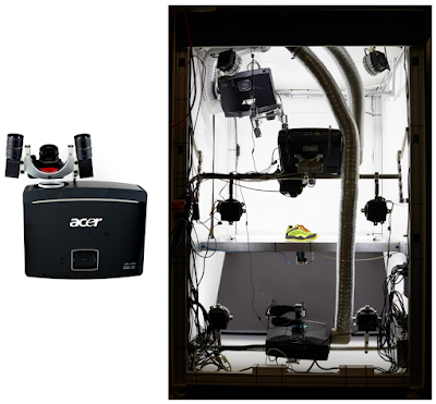 |
| The scanning rig used to capture 3D models. |
| A shoe being scanned (left). Images are captured from several directions with different patterns of light and color. A shadow passing over an object (right) illustrates how a 3D shape can be captured with an off-axis view of a shadow edge. |
Simulation Model Conversion
The early internal scanned models used protocol buffer metadata, high-resolution visuals, and formats that were not suitable for simulation. For some objects, physical properties, such as mass, were captured by weighing the objects at scanning time, but surface properties, such as friction or deformation, were not represented.
So, following data collection, we built an automated pipeline to solve these issues and enable the use of scanned models in simulation systems. The automated pipeline filters out invalid or duplicate objects, automatically assigns object names using text descriptions of the objects, and eliminates object mesh scans that do not meet simulation requirements. Next, the pipeline estimates simulation properties (e.g., mass and moment of inertia) from shape and volume, constructs collision volumes, and downscales the model to a usable size. Finally, the pipeline converts each model to SDF format, creates thumbnail images, and packages the model for use in simulation systems.
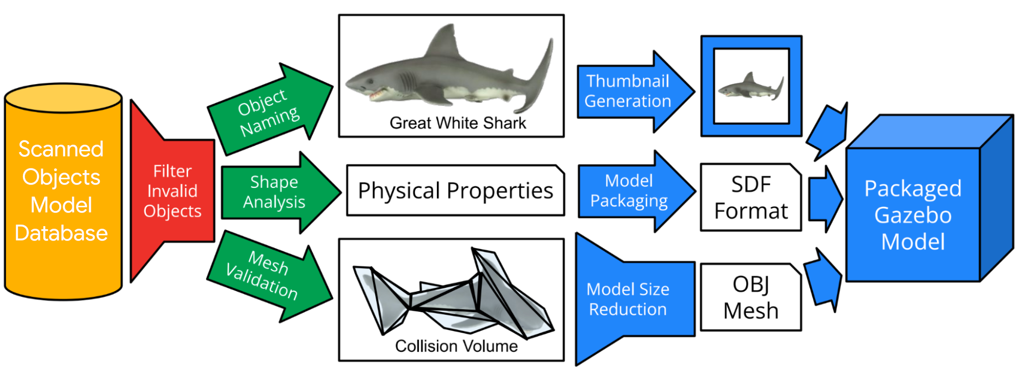 |
| The pipeline filters models that are not suitable for simulation, generates collision volumes, computes physical properties, downsamples meshes, generates thumbnails, and packages them all for use in simulation systems. |
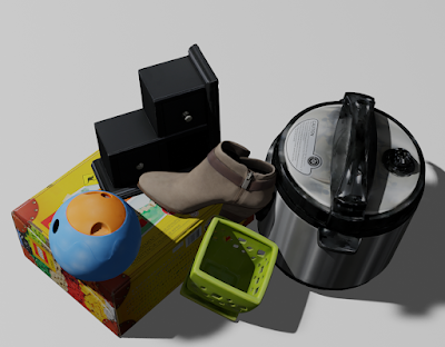 |
| A collection of Scanned Object models rendered in Blender. |
The output of this pipeline is a simulation model in an appropriate format with a name, mass, friction, inertia, and collision information, along with searchable metadata in a public interface compatible with our open-source hosting on Open Robotics’ Gazebo.
The output objects are represented as SDF models that refer to Wavefront OBJ meshes averaging 1.4 Mb per model. Textures for these models are in PNG format and average 11.2 Mb. Together, these provide high resolution shape and texture.
Impact
The Scanned Objects dataset contains 1030 scanned objects and their associated metadata, totaling 13 Gb, licensed under the CC-BY 4.0 License. Because these models are scanned rather than modeled by hand, they realistically reflect real object properties, not idealized recreations, reducing the difficulty of transferring learning from simulation to the real world.
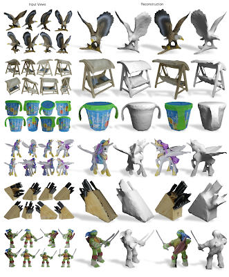 |
| Input views (left) and reconstructed shape and texture from two novel views on the right (figure from Differentiable Stereopsis). |
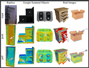 |
| Visualized action scoring predictions over three real-world 3D scans from the Replica dataset and Scanned Objects (figure from Where2Act). |
The Scanned Objects dataset has already been used in over 25 papers across as many projects, spanning computer vision, computer graphics, robot manipulation, robot navigation, and 3D shape processing. Most projects used the dataset to provide synthetic training data for learning algorithms. For example, the Scanned Objects dataset was used in Kubric, an open-sourced generator of scalable datasets for use in over a dozen vision tasks, and in LAX-RAY, a system for searching shelves with lateral access X-rays to automate the mechanical search for occluded objects on shelves.
We hope that the Scanned Objects dataset will be used by more robotics and simulation researchers in the future, and that the example set by this dataset will inspire other owners of 3D model repositories to make them available for researchers everywhere. If you would like to try it yourself, head to Gazebo and start browsing!
Acknowledgments
The authors thank the Scanned Objects team, including Peter Anderson-Sprecher, J.J. Blumenkranz, James Bruce, Ken Conley, Katie Dektar, Charles DuHadway, Anthony Francis, Chaitanya Gharpure, Topraj Gurung, Kristy Headley, Ryan Hickman, John Isidoro, Sumit Jain, Brandon Kinman, Greg Kline, Mach Kobayashi, Nate Koenig, Kai Kohlhoff, James Kuffner, Thor Lewis, Mike Licitra, Lexi Martin, Julian (Mac) Mason, Rus Maxham, Pascal Muetschard, Kannan Pashupathy, Barbara Petit, Arshan Poursohi, Jared Russell, Matt Seegmiller, John Sheu, Joe Taylor, Vincent Vanhoucke, Josh Weaver, and Tommy McHugh.
Special thanks go to Krista Reymann for organizing this project, helping write the paper, and editing this blogpost, James Bruce for the scanning pipeline design and Pascal Muetschard for maintaining the database of object models.


")

 Learn about how the Visual Components NVIDIA Omniverse Connector creates a simulation solution for the manufacturing industry to resolve operational and planning challenges.


