I was wondering ,when creating an image classifer with tflite-model-maker, what is the optimal size for the images in the datasets . Thanks 🙂
submitted by /u/DrakenZA
[visit reddit] [comments]
 DataBloom
I was wondering ,when creating an image classifer with tflite-model-maker, what is the optimal size for the images in the datasets . Thanks 🙂
submitted by /u/DrakenZA
[visit reddit] [comments]
Hi all. I am trying to train a neural net to perform handwritten character recognition, and have attached the relevant code below. I’m training 28×28 size characters with the EMNIST dataset. No matter how what I change the batch size to, when I try to train the model, I always get a similar error at the bottom. Does anyone know how to fix this? Thank you for the help!
def load_dataset(): X_train = X_train.reshape((X_train.shape[0], 28, 28, 1)) X_test = X_test.reshape((X_test.shape[0], 28, 28, 1)) y_train = to_categorical(y_train) y_test = to_categorical(y_test) return X_train, y_train, X_test, y_test def prep_pixels(train, test): train_norm = train.astype('float32') test_norm = test.astype('float32') train_norm = train_norm/255.0 test_norm = test_norm/255.0 return train_norm, test_norm def define_model(): model = Sequential() model.add(Conv2D(32, (3,3), activation = 'relu', kernel_initializer = 'he_uniform', input_shape = (28, 28, 1))) model.add(MaxPooling2D((2,2))) model.add(Flatten()) model.add(Dense(100, activation = 'relu', kernel_initializer = 'he_uniform')) model.add(Dense(46, activation = 'softmax')) opt = SGD(learning_rate = 0.01, momentum = 0.9) model.compile(optimizer = opt, loss = 'categorical_crossentropy', metrics = ['accuracy']) return model def evaluate_model(dataX, dataY, xtest, ytest, n_folds = 5): model = define_model() history = model.fit(dataX, dataY, epochs = 4, batch_size = 64, validation_data = (xtest, ytest)) _, acc = model.evaluate(dataX, dataY, verbose=0) scores.append(acc) histories.append(history)
ValueError: Shapes (64, 1) and (64, 46) are incompatible
EDIT: Fixed some bugs, but still have the same error
submitted by /u/landshark223344
[visit reddit] [comments]
I have been following the tensorflow examples on how to set up a model for pruning and quantise it in order to improve inference. What I noticed however was:
1) the sparse model resulted from pruning has no faster inference benefits
2) the quantisation makes the model even slower (I know that this is probably due to TFlite not being optimised for x86).
What is the method you use to prune your models?
submitted by /u/ats678
[visit reddit] [comments]
I have two classes and trying to build Tensorflow ranking model
when i run model.fit(cached_train, epochs=3), i get error
ValueError: The first argument to `Layer.call` must always be passed
class ProdRankingModel(tf.keras.Model):
def __init__(self):
super().__init__()
embedding_dimension = 32
self.user_embeddings = tf.keras.Sequential([
tf.keras.layers.StringLookup(
vocabulary=unique_user_ids, mask_token=None),
tf.keras.layers.Embedding(len(unique_user_ids) + 1, embedding_dimension)])
self.prod_embeddings = tf.keras.Sequential([
tf.keras.layers.StringLookup(
vocabulary=unique_items, mask_token=None),
tf.keras.layers.Embedding(len(unique_items) + 1, embedding_dimension)
])
# Compute predictions.
self.ratings = tf.keras.Sequential([
tf.keras.layers.Dense(256, activation=”relu”),
tf.keras.layers.Dense(64, activation=”relu”),
tf.keras.layers.Dense(1)
])
def call(self, inputs):
user_id, products = inputs
user_embedding = self.user_embeddings(user_id)
product_embedding = self.prod_embeddings(products)
return self.ratings(tf.concat([user_embedding, product_embedding], axis=1))
class ProductModel(tfrs.models.Model):
def __init__(self):
super().__init__()
self.prodranking_model: tf.keras.Model = ProdRankingModel()
self.task: tf.keras.layers.Layer = tfrs.tasks.Ranking(
loss = tf.keras.losses.MeanSquaredError(),
metrics=[tf.keras.metrics.RootMeanSquaredError()]
)
def call(self, features: Dict[str, tf.Tensor]) -> tf.Tensor:
return self.prodranking_model(
(features[“user_id”], features[“prod_name”]))
def compute_loss(self, features: Dict[Text, tf.Tensor], training=False) -> tf.Tensor:
labels = features.pop(“prod_count”)
rating_predictions = self(features)
# The task computes the loss and the metrics.
return self.task(labels=labels, predictions=rating_predictions)
submitted by /u/TimelyAbbreviations1
[visit reddit] [comments]
Hi! I’m building a CNN for the first time for a university project: the idea is to classify images coming from 10 animal classes (taken from ImageNet).
Anybody willing to give me some advice about my model? Here’s my model:
model = Sequential() model.add(layers.InputLayer(input_shape=(224,224,3))) model.add(layers.BatchNormalization()) model.add(layers.Conv2D(64,(3,3), activation='relu')) model.add(layers.BatchNormalization()) model.add(layers.Conv2D(64,(3,3),activation='relu')) model.add(layers.BatchNormalization()) model.add(layers.Conv2D(128,(3,3),activation='relu')) model.add(layers.BatchNormalization()) model.add(layers.Conv2D(256,(3,3),activation='relu')) model.add(layers.AvgPool2D(2,2)) model.add(layers.Flatten(name='features_layer')) model.add(layers.Dense(10, activation='softmax'))
Training Loss keeps decreasing and training accuracy keeps improving (and even converges to 1) but after ~10 epochs I’m stuck around 0.5 validation accuracy. The actual dataset contains 2500 images, and I tried both with a 0.2 validation split and 0.3. Using 0.2 leads to more stable results, but reach 0.5 val_accuracy more slowly. I can try augmenting my dataset (creating some slightly modified copies of the images I have), but the training time increases quite a lot, and I would like to be reasonably sure that my model is good (at least on theory) before training with high number of epochs and new expanded dataset.
Is the overall structure of my net correct? Some questions:
Sorry for the bunch of ‘noob’ questions, I hope you’ll understand my perplexity. As I said, it is my first time dealing with building a CNN myself and I feel that even real ‘general’ suggestions might help. I would really appreciate any advice c:
submitted by /u/synchro-azel
[visit reddit] [comments]
submitted by /u/blevlabs
[visit reddit] [comments]
I faced an error when I was building Tensorflow from the source with my laptop. It has only 8GB RAM and out of memory is the reason for the error. I’m going to buy a new laptop but I’m not sure how much memory Tensorflow requires. MacBook Air is one of the candidates. I would be happy if I know something about it. Thanks.
submitted by /u/SubstantialSwimmer4
[visit reddit] [comments]
 Learn about our joint effort in porting the ILT engine to GPU. We also identify future areas for EDA and mask inspection tool vendors to address for ILT to be adopted at logic foundries.
Inverse lithography technology (ILT) was first implemented and demonstrated in early 2003. It was created by Danping Peng, while he worked as an engineer at Luminescent Technologies Inc., a startup company founded by professors Stanley Osher and Eli Yabonovitch from UCLA and entrepreneurs Dan Abrams and Jack Herrik.
At that time, ILT was a revolutionary solution that showed far superior process-window than conventional Manhattan mask shapes used in lithography patterning. Unlike Manhattan mask shapes that are rectilinear, ILT’s advantage lies in its curvilinear mask shapes.
Following its development, ILT was demonstrated as a viable lithography technique in actual wafer printing at several memory and logic foundries. However, technical and economic factors hindered the adoption of ILT:
Due to these reasons, ILT’s usage was largely used in memory foundries for cell-array printing and in logic foundries as hot-spot repair or used to benchmark and improve the traditional optical proximity correction (OPC).
Fast forward to 20 years later and there is a different semiconductor landscape today. The challenges in patterning feature sizes at 7nm and lower require far greater accuracy and process margin. Thus, the ability to produce curvilinear mask shapes in ILT becomes increasingly critical to overcoming these wafer production limitations.
Today’s advancement in lithographic simulation on GPU achieved speedups of over 10x more than traditional CPU computation, with machine learning (ML) providing further speedup of the ILT model by learning from existing solutions.
Multi-Beam mask writers could also write masks of any complexity in fixed time and it has been successfully used in HVM.
Finally, next-generation lithography scanners are becoming increasingly expensive, therefore extracting value and performance from existing scanners through ILT was a more appealing option.
Through GPU computing and ML, the deployment of ILT for full-chip applications is becoming a reality. It is expected to play a key role in pushing the frontiers of mask patterning and defect inspection technologies.
To use ILT successfully in a logic foundry environment, you must address the issues that prevented its mass adoption:
ILT requires a long computation time due to the complexity of curvilinear mask shapes. Fortunately, recent progress in GPU computing performance and deep learning (DL) has significantly reduced the amount of time required to solve these complex computation algorithms.
Second, mask-rule checking (MRC) specific to curvilinear OPC must be addressed as mask shops need a method of verifying whether the incoming mask data is manufacturable. This is especially so for curvilinear mask shapes, as they are more challenging to verify than rectilinear mask shapes since simple width and space checks are no longer applicable in curvilinear masks.
To address MRC, the industry is converging to using simplified rules, such as minimal CD/Space, minimal area for holes and islands, and smoothness of mask edge (upper-bound for curvature).
Lastly, layout file sizes generated by ILT are unacceptably large compared to conventional rectilinear shapes. The increased size represents a significantly increased cost of data generation, storage, transfer, and use in manufacturing.
To solve this, EDA vendors have proposed various solutions, and a working group was formed to work on a common file format supported by all stakeholders (EDA vendors, tool suppliers, and foundries).
Our close partnership with EDA vendors and NVIDIA has resulted in a home-grown ILT solution. Using the NVIDIA GPU platform, we successfully ported most of the simulation and ILT engine using NVIDIA SDKs and libraries:
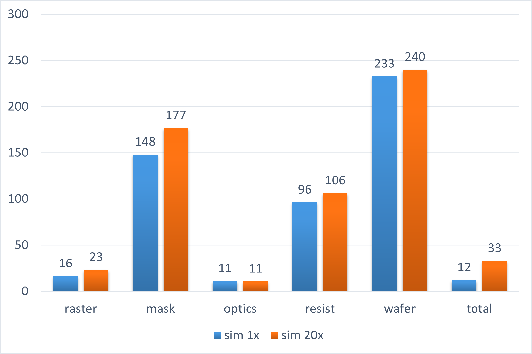
On NVIDIA V100 32-GB GPUs, we demonstrated over 10x speedup in ILT computations as compared to our typical CPU runs. In many key components of the optical and resist modeling, we saw an over 20x speedup.
The encouraging results have led to further developments. We are currently in the process of production scale calibration and testing of key layers using our in-house ILT engine on an NVIDIA A100 80-GB GPU cluster.
Advanced chip design increasingly relies on expensive simulations: from circuit performance and timing to thermal dissipation. When it comes to manufacturing, OPC/ILT requires a huge amount of computing power, which is expected to increase as we rapidly progress towards the next node.
Employing HPC with GPUs as well as the entire software stack, consistent with the observation in Huang’s Law, will be the key component to successfully rolling out future generation chips on schedule. More specifically, a unified acceleration architecture for HPC + Rendering (Computer Graphics) + ML/DL will enable better chips to be designed and manufactured, which in turn contributes to improving the speed and efficiency of mask patterning and defect detection applications.
In other words, it’s an iterative process of using GPUs to design faster and better GPUs.
To enable the rapid adoption of ILT masks in HVM, all stakeholders must participate in partnerships and collaborations.
There’s no doubt that curvilinear ILT mask designs provide circuit designers with greater freedom and creativity to create circuits with better performance while enabling better process margins with greatly simplified design rules. The benefits of using curvilinear design will have a significant impact on the semiconductor industry and ILT will be the key enabler to the future development of process nodes.
I have converted 2 csv files into arrays in the hopes that I can create a positive training sample. Could someone help me find a way to combine anchors and matches, so that they are a positive training sample. This would be hugely appreciated as I am quite stuck.
## Convert csv to tensor
anchor = train
anchors = np.array(anchor)
match = train2
matches = np.array(match)
# Create positive training sample
??????
submitted by /u/MinuteBeginning9933
[visit reddit] [comments]
I read about Grappler and that it can optimize TF models, which is an interesting feature.
I use keras to create, train and save models, and also convert them to tflite in order to deploy them on other systems. My question is, whether this optimization is already integrated into keras and / or the tflite conversion.
It seems like quite a big topic to get into, so if it already happens automatically, I don’t want to spend so much time on it.
submitted by /u/norobot12
[visit reddit] [comments]