Posted by Andrew M Dai and Nan Du, Research Scientists, Google Research, Brain Team
Large language models (e.g., GPT-3) have many significant capabilities, such as performing few-shot learning across a wide array of tasks, including reading comprehension and question answering with very few or no training examples. While these models can perform better by simply using more parameters, training and serving these large models can be very computationally intensive. Is it possible to train and use these models more efficiently?
In pursuit of that question, today we introduce the Generalist Language Model (GLaM), a trillion weight model that can be trained and served efficiently (in terms of computation and energy use) thanks to sparsity, and achieves competitive performance on multiple few-shot learning tasks. GLaM’s performance compares favorably to a dense language model, GPT-3 (175B) with significantly improved learning efficiency across 29 public NLP benchmarks in seven categories, spanning language completion, open-domain question answering, and natural language inference tasks.
Dataset
To build GLaM, we began by building a high-quality 1.6 trillion token dataset containing language usage representative of a wide range of downstream use-cases for the model. Web pages constitute the vast quantity of data in this unlabelled corpus, but their quality ranges from professional writing to low-quality comment and forum pages. We then developed a text quality filter that was trained on a collection of text from Wikipedia and books (both of which are generally higher quality sources) to determine the quality of the content for a webpage. Finally, we applied this filter to generate the final subset of webpages and combined this with books and Wikipedia to create the final training dataset.
Model and Architecture
GLaM is a mixture of experts (MoE) model, a type of model that can be thought of as having different submodels (or experts) that are each specialized for different inputs. The experts in each layer are controlled by a gating network that activates experts based on the input data. For each token (generally a word or part of a word), the gating network selects the two most appropriate experts to process the data. The full version of GLaM has 1.2T total parameters across 64 experts per MoE layer with 32 MoE layers in total, but only activates a subnetwork of 97B (8% of 1.2T) parameters per token prediction during inference.
 |
| The architecture of GLaM where each input token is dynamically routed to two selected expert networks out of 64 for prediction. |
Similar to the GShard MoE Transformer, we replace the single feedforward network (the simplest layer of an artificial neural network, “Feedforward or FFN” in the blue boxes) of every other transformer layer with a MoE layer. This MoE layer has multiple experts, each a feedforward network with identical architecture but different weight parameters. Even though this MoE layer has many more parameters, the experts are sparsely activated, meaning that for a given input token, only two experts are used, giving the model more capacity while limiting computation. During training, each MoE layer’s gating network is trained to use its input to activate the best two experts for each token, which are then used for inference. For a MoE layer of E experts, this essentially provides a collection of E×(E-1) different feedforward network combinations (instead of one as in the classic Transformer architecture), leading to more computational flexibility.
The final learned representation of a token will be the weighted combination of the outputs from the two experts. This allows different experts to activate on different types of inputs. To enable scaling to larger models, each expert within the GLaM architecture can span multiple computational devices. We use the GSPMD compiler backend to solve the challenges in scaling the experts and train several variants (based on expert size and number of experts) of this architecture to understand the scaling effects of sparsely activated language models.
Evaluation
We use a zero-shot and one-shot setting where the tasks are never seen during training. The benchmarks for evaluation include (1) cloze and completion tasks [1,2,3]; (2) Open-domain question answering [4,5,6]; (3) Winograd-style tasks [7,8]; (4) commonsense reasoning [9,10,11]; (5) in-context reading comprehension [12,13,14,15,16]; (6) the SuperGLUE tasks; and (7) natural language inference [17]. In total, there are eight natural language generation tasks (NLG) where the generated phrases are evaluated against the ground truth targets via Exact Match (EM) accuracy and F1 measure, and 21 language understanding tasks (NLU) where the prediction from several options is chosen via conditional log-likelihood. Some tasks have variants and SuperGLUE consists of multiple tasks. Both EM accuracy and F1 are scaled from 0 to 100 across all our results and averaged for the NLG score below. The NLU score is an average of accuracy and F1 scores.
Results
GLaM reduces to a basic dense Transformer-based language model architecture when each MoE layer only has one expert. In all experiments, we adopt the notation of (base dense model size) / (number of experts per MoE layer) to describe the GLaM model. For example, 1B/64E represents the architecture of a 1B parameter dense model with every other layer replaced by a 64 expert MoE layer. In the following sections, we explore GLaM’s performance and scaling properties, including baseline dense models trained on the same datasets. Compared with the recently announced Megatron-Turing model, GLaM is on-par on the seven respective tasks if using a 5% margin, while using 5x less computation during inference.
Below, we show the 1.2T-parameter sparsely activated model (GLaM) achieved higher results on average and on more tasks than the 175B-parameter dense GPT-3 model while using less computation during inference.
 |
| Average score for GLaM and GPT-3 on NLG (left) and NLU (right) tasks (higher is better). |
Below we show a summary of the performance on 29 benchmarks compared to the dense model (GPT-3, 175B). GLaM exceeds or is on-par with the performance of the dense model on almost 80% of zero-shot tasks and almost 90% of one-shot tasks.
| Evaluation |
Higher (>+5%) |
On-par (within 5%) |
Lower (<-5%) |
| Zero-shot |
13 |
11 |
5 |
| One-shot |
14 |
10 |
5 |
Moreover, while the full version of GLaM has 1.2T total parameters, it only activates a subnetwork of 97B parameters (8% of 1.2T) per token during inference.
| |
GLaM (64B/64E) |
GPT-3 (175B) |
| Total Parameters |
1.162T |
0.175T |
| Activated Parameters |
0.097T |
0.175T |
Scaling Behavior
GLaM has two ways to scale: 1) scale the number of experts per layer, where each expert is hosted within one computation device, or 2) scale the size of each expert to go beyond the limit of a single device. To evaluate the scaling properties, we compare the respective dense model (FFN layers instead of MoE layers) of similar FLOPS per token at inference time.
 |
| Average zero-shot and one-shot performance by increasing the size of each expert. The FLOPS per token prediction at inference time increases as the expert size grows. |
As shown above, performance across tasks scales with the size of the experts. GLaM sparsely activated models also perform better than dense models for similar FLOPs during inference for generation tasks. For understanding tasks, we observed that they perform similarly at smaller scales, but sparsely activated models outperform at larger scales.
Data Efficiency
Training large language models is computationally intensive, so efficiency improvements are useful to reduce energy consumption.
Below we show the computation costs for the full version of GLaM.
 |
| Computation cost in GFLOPS both for inference, per token (left) and for training (right). |
These compute costs show that GLaM uses more computation during training since it trains on more tokens, but uses significantly less computation during inference. We show comparisons using different numbers of tokens to train below.
We also evaluated the learning curves of our models compared to the dense baseline.
 |
| Average zero-shot and one-shot performance of sparsely-activated and dense models on eight generative tasks as more tokens are processed in training. |
 |
| Average zero-shot and one-shot performance of sparsely-activated and dense models on 21 understanding tasks as more tokens are processed in training. |
The results above show that sparsely activated models need to train with significantly less data than dense models to reach similar zero-shot and one-shot performance, and if the same amount of data is used, sparsely activated models perform significantly better.
Finally, we assessed the energy efficiency of GLaM.
 |
| Comparison of power consumption during training. |
While GLaM uses more computation during training, thanks to the more efficient software implementation powered by GSPMD and the advantage of TPUv4, it uses less power to train than other models.
Conclusions
Our large-scale sparsely activated language model, GLaM, achieves competitive results on zero-shot and one-shot learning and is a more efficient model than prior monolithic dense counterparts. We also show quantitatively that a high-quality dataset is essential for large language models. We hope that our work will spark more research into compute-efficient language models.
Acknowledgements
We wish to thank Claire Cui, Zhifeng Chen, Yonghui Wu, Quoc Le, Macduff Hughes, Fernando Pereira, Zoubin Ghahramani and Jeff Dean for their support and invaluable input. Special thanks to our collaborators: Yanping Huang, Simon Tong, Yanqi Zhou, Yuanzhong Xu, Dmitry Lepikhin, Orhan Firat, Maxim Krikun, Tao Wang, Noam Shazeer, Barret Zoph, Liam Fedus, Maarten Bosma, Kun Zhang, Emma Wang, David Patterson, Zongwei Zhou, Naveen Kumar, Adams Yu, Laurent Shafey, Jonathan Shen, Ben Lee, Anmol Gulati, David So, Marie Pellat, Kevin Robinson, Kathy Meier-Hellstern, Aakanksha Chowdhery, Sharan Narang, Erica Moreira and Eric Ni for helpful discussions and inspirations; and the larger Google Research team. We would also like to thank Tom Small for the animated figure used in this post.

 The groundbreaking technology uses an optical metasurface and machine-learning algorithms to produce high-quality color images with a wide field of view.
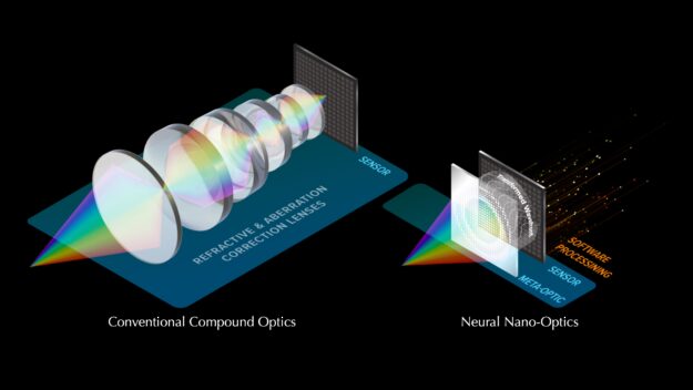


 NVIDIA has partnered with iD Tech to create the Artificial Intelligence and Machine Learning certification program, a boot-camp style course for teens.
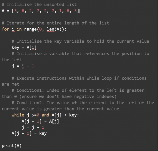
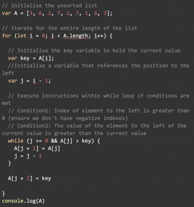
 Learn a step-by-step breakdown of sorting algorithms. A fundamental tools used in data science.
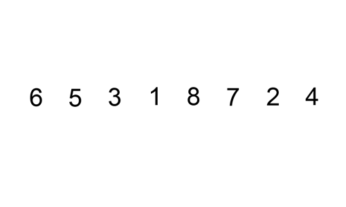
 The Jetson Project of the Month simplifies home automation projects using a combination of DeepStack and Home Assistant along with the NVIDIA Jetson.