Posted by Kihyuk Sohn and Chun-Liang Li, Research Scientists, Google Cloud
Anomaly detection (sometimes called outlier detection or out-of-distribution detection) is one of the most common machine learning applications across many domains, from defect detection in manufacturing to fraudulent transaction detection in finance. It is most often used when it is easy to collect a large amount of known-normal examples but where anomalous data is rare and difficult to find. As such, one-class classification, such as one-class support vector machine (OC-SVM) or support vector data description (SVDD), is particularly relevant to anomaly detection because it assumes the training data are all normal examples, and aims to identify whether an example belongs to the same distribution as the training data. Unfortunately, these classical algorithms do not benefit from the representation learning that makes machine learning so powerful. On the other hand, substantial progress has been made in learning visual representations from unlabeled data via self-supervised learning, including rotation prediction and contrastive learning. As such, combining one-class classifiers with these recent successes in deep representation learning is an under-explored opportunity for the detection of anomalous data.
In “Learning and Evaluating Representations for Deep One-class Classification”, presented at ICLR 2021, we outline a 2-stage framework that makes use of recent progress on self-supervised representation learning and classic one-class algorithms. The algorithm is simple to train and results in state-of-the-art performance on various benchmarks, including CIFAR, f-MNIST, Cat vs Dog and CelebA. We then follow up on this in “CutPaste: Self-Supervised Learning for Anomaly Detection and Localization”, presented at CVPR 2021, in which we propose a new representation learning algorithm under the same framework for a realistic industrial defect detection problem. The framework achieves a new state-of-the-art on the MVTec benchmark.
A Two-Stage Framework for Deep One-Class Classification
While end-to-end learning has demonstrated success in many machine learning problems, including deep learning algorithm designs, such an approach for deep one-class classifiers often suffer from degeneration in which the model outputs the same results regardless of the input.
To combat this, we apply a two stage framework. In the first stage, the model learns deep representations with self-supervision. In the second stage, we adopt one-class classification algorithms, such as OC-SVM or kernel density estimator, using the learned representations from the first stage. This 2-stage algorithm is not only robust to degeneration, but also enables one to build more accurate one-class classifiers. Furthermore, the framework is not limited to specific representation learning and one-class classification algorithms — that is, one can easily plug-and-play different algorithms, which is useful if any advanced approaches are developed.
 |
| A deep neural network is trained to generate the representations of input images via self-supervision. We then train one-class classifiers on the learned representations. |
Semantic Anomaly Detection
We test the efficacy of our 2-stage framework for anomaly detection by experimenting with two representative self-supervised representation learning algorithms, rotation prediction and contrastive learning.
Rotation prediction refers to a model’s ability to predict the rotated angles of an input image. Due to its promising performance in other computer vision applications, the end-to-end trained rotation prediction network has been widely adopted for one-class classification research. The existing approach typically reuses the built-in rotation prediction classifier for learning representations to conduct anomaly detection, which is suboptimal because those built-in classifiers are not trained for one-class classification.
In contrastive learning, a model learns to pull together representations from transformed versions of the same image, while pushing representations of different images away. During training, as images are drawn from the dataset, each is transformed twice with simple augmentations (e.g., random cropping or color changing). We minimize the distance of the representations from the same image to encourage consistency and maximize the distance between different images. However, usual contrastive learning converges to a solution where all the representations of normal examples are uniformly spread out on a sphere. This is problematic because most of the one-class algorithms determine the outliers by checking the proximity of a tested example to the normal training examples, but when all the normal examples are uniformly distributed in an entire space, outliers will always appear close to some normal examples.
To resolve this, we propose distribution augmentation (DA) for one-class contrastive learning. The idea is that instead of learning representations from the training data only, the model learns from the union of the training data plus augmented training examples, where the augmented examples are considered to be different from the original training data. We employ geometric transformations, such as rotation or horizontal flip, for distribution augmentation. With DA, the training data is no longer uniformly distributed in the representation space because some areas are occupied by the augmented data.
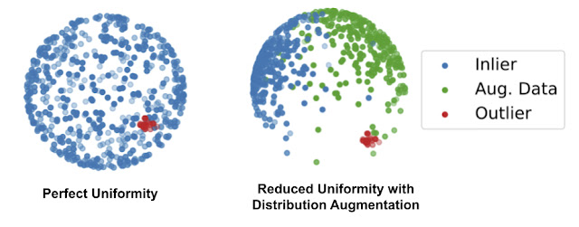 |
| Left: Illustrated examples of perfect uniformity from the standard contrastive learning. Right: The reduced uniformity by the proposed distribution augmentation (DA), where the augmented data occupy the space to avoid the uniform distribution of the inlier examples (blue) throughout the whole sphere. |
We evaluate the performance of one-class classification in terms of the area under receiver operating characteristic curve (AUC) on the commonly used datasets in computer vision, including CIFAR10 and CIFAR-100, Fashion MNIST, and Cat vs Dog. Images from one class are given as inliers and those from remaining classes are given as outliers. For example, we see how well cat images are detected as anomalies when dog images are inliers.
| |
CIFAR-10 |
CIFAR-100 |
f-MNIST |
Cat v.s. Dog |
| Ruff et al. (2018) |
64.8 |
– |
– |
– |
| Golan and El-Yaniv (2018) |
86.0 |
78.7 |
93.5 |
88.8 |
| Bergman and Hoshen (2020) |
88.2 |
– |
94.1 |
– |
| Hendrycks et al. (2019) |
90.1 |
– |
– |
– |
| Huang et al. (2019) |
86.6 |
78.8 |
93.9 |
– |
| 2-stage framework: rotation prediction |
91.3±0.3 |
84.1±0.6 |
95.8±0.3 |
86.4±0.6 |
| 2-stage framework: contrastive (DA) |
92.5±0.6 |
86.5±0.7 |
94.8±0.3 |
89.6±0.5 |
| Performance comparison of one-class classification methods. Values are the mean AUCs and their standard deviation over 5 runs. AUC ranges from 0 to 100, where 100 is perfect detection. |
Given the suboptimal built-in rotation prediction classifiers typically used for rotation prediction approaches, it’s notable that simply replacing the built-in rotation classifier used in the first stage for learning representations with a one-class classifier at the second stage of the proposed framework significantly boosts the performance, from 86 to 91.3 AUC. More generally, the 2-stage framework achieves state-of-the-art performance on all of the above benchmarks.
With classic OC-SVM, which learns the area boundary of representations of normal examples, the 2-stage framework results in higher performance than existing works as measured by image-level AUC.
Texture Anomaly Detection for Industrial Defect Detection
In many real-world applications of anomaly detection, the anomaly is often defined by localized defects instead of entirely different semantics (i.e., being different in general). For example, the detection of texture anomalies is useful for detecting various kinds of industrial defects.
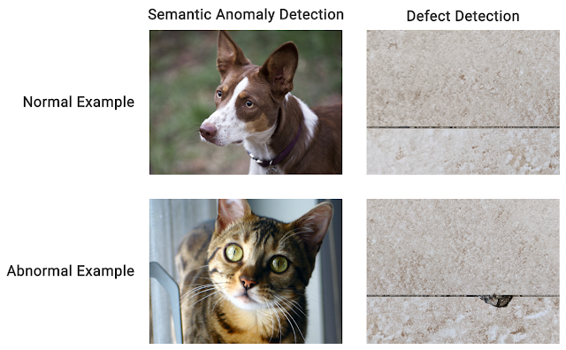 |
| The examples of semantic anomaly detection and defect detection. In semantic anomaly detection, the inlier and outlier are different in general, (e.g., one is a dog, the other a cat). In defect detection, the semantics for inlier and outlier are the same (e.g., they are both tiles), but the outlier has a local anomaly. |
While learning representations with rotation prediction and distribution-augmented contrastive learning have demonstrated state-of-the-art performance on semantic anomaly detection, those algorithms do not perform well on texture anomaly detection. Instead, we explored different representation learning algorithms that better fit the application.
In our second paper, we propose a new self-supervised learning algorithm for texture anomaly detection. The overall anomaly detection follows the 2-stage framework, but the first stage, in which the model learns deep image representations, is specifically trained to predict whether the image is augmented via a simple CutPaste data augmentation. The idea of CutPaste augmentation is simple — a given image is augmented by randomly cutting a local patch and pasting it back to a different location of the same image. Learning to distinguish normal examples from CutPaste-augmented examples encourages representations to be sensitive to local irregularity of an image.
 |
| The illustration of learning representations by predicting CutPaste augmentations. Given an example, the CutPaste augmentation crops a local patch, then pasties it to a randomly selected area of the same image. We then train a binary classifier to distinguish the original image and the CutPaste augmented image. |
We use MVTec, a real-world defect detection dataset with 15 object categories, to evaluate the approach above.
| Image-level anomaly detection performance (in AUC) on the MVTec benchmark. |
Besides image-level anomaly detection, we use the CutPaste method to locate where the anomaly is, i.e., “patch-level” anomaly detection. We aggregate the patch anomaly scores via upsampling with Gaussian smoothing and visualize them in heatmaps that show where the anomaly is. Interestingly, this provides decently improved localization of anomalies. The below table shows the pixel-level AUC for localization evaluation.
Autoencoder
(Bergmann et al., 2019) |
FCDD
(Ruff et al., 2020) |
Rotation Prediction |
Contrastive (DA) |
CutPaste |
| 86.0 |
92.0 |
93.0 |
90.4 |
96.0 |
| Pixel-level anomaly localization performance (in AUC) comparison between different algorithms on the MVTec benchmark. |
Conclusion
In this work we introduce a novel 2-stage deep one-class classification framework and emphasize the importance of decoupling building classifiers from learning representations so that the classifier can be consistent with the target task, one-class classification. Moreover, this approach permits applications of various self-supervised representation learning methods, attaining state-of-the-art performance on various applications of visual one-class classification from semantic anomaly to texture defect detection. We are extending our efforts to build more realistic anomaly detection methods under the scenario where training data is truly unlabeled.
Acknowledgements
We gratefully acknowledge the contribution from other co-authors, including Jinsung Yoon, Minho Jin and Tomas Pfister. We release the code in our GitHub repository.


 3D deep learning researchers can build on more cutting edge algorithms and simplify their workflows with the latest version of the Kaolin PyTorch Library.
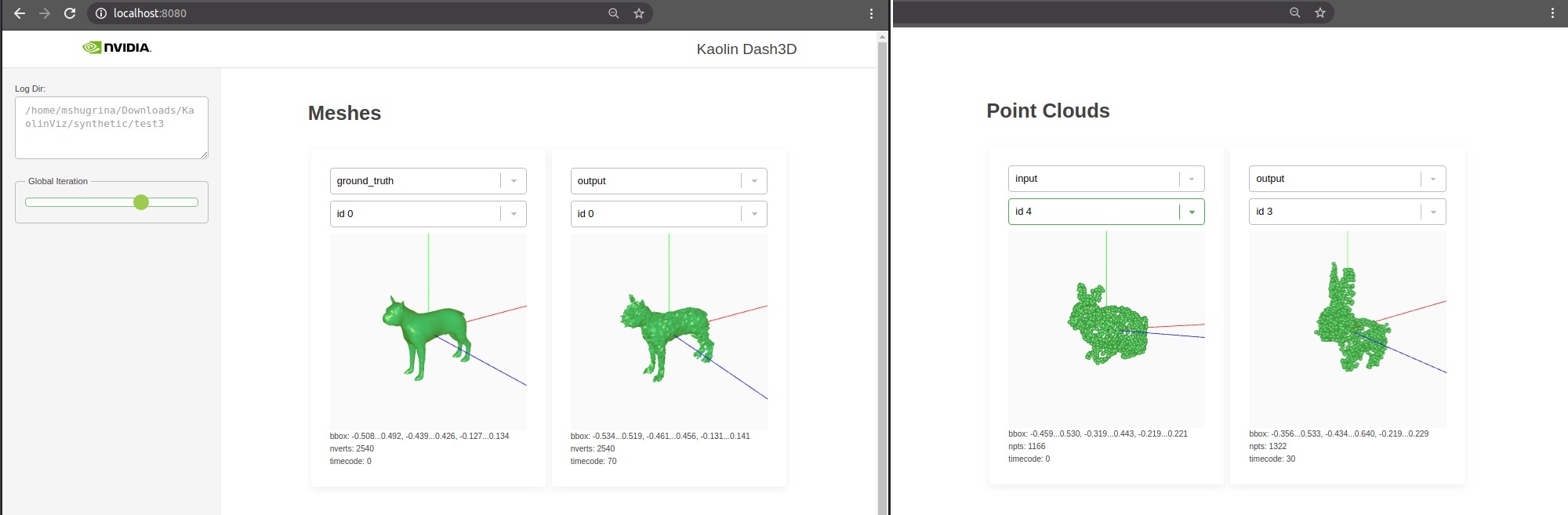
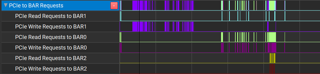
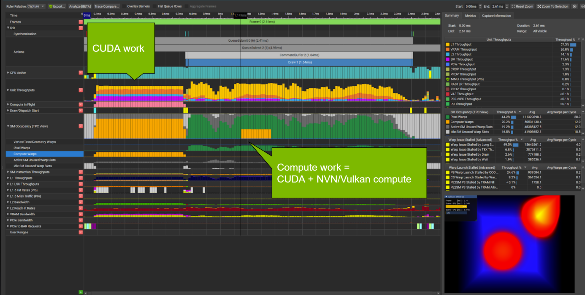
 Learn about the latest release of Nsight Graphics 2021.4, an all-in-one graphics debugger and profiler to help game developers get the most out of NVIDIA hardware.
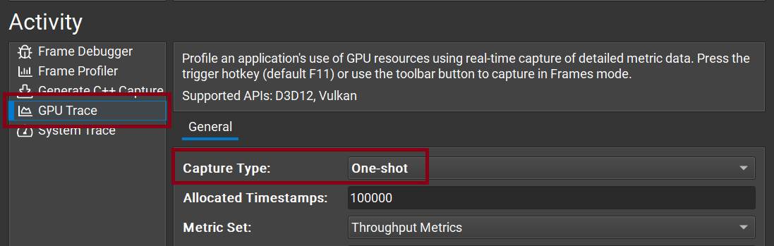


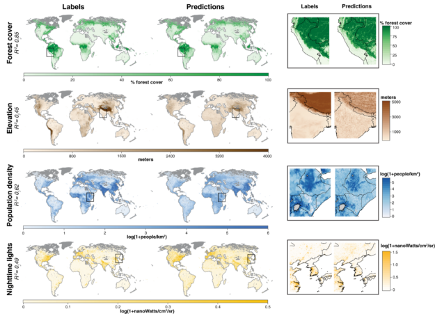
 New research creates a low-cost and easy-to-use machine learning model to analyze streams of data from earth-imaging satellites.