I have been working on two codes, one in TF1, the other one in TF2. I did some research about the TensorFlow architecture the difference between these two, maybe you could check if my understanding is correct?
In version 1, graphs need to be created manually by the user. In version 2, the API has been made more user-friendly and the graph creation is now automated in Keras. Has Keras been created explicitly for TensorFlow 2, or does it exist independently from it?
The eager execution mode basically breaks the graph approach to create a more “classical” computation scheme. It is used per default in pure high-level TensorFlow, since here the computations have a smaller impact on performance. On the other hand, in Keras, eager mode is switched off and behaves more or less like TF1. Is this correct?
I have extracted audio embeddings from Google Audioset corpus.
Now, I want to use these audio embeddings for training my own model (CNN). I have some confusion about these audio embeddings.
Should I extract STFT and MFCC from the audio embeddings? If so, how can I do that (any way to use librosa?)? Or, are the audio embeddings already transformed to MFCC?
What should be the best way to split the audio set corpus into train, test and validate datasets? They are if Tfrecord format and each tfrecord file contain various segment of audio clips having different class labels.
If I want to work on selective class labels (such as rowing, or car sound), what should be the best way to extract the selective audio segments?
Also, please share some helpful resources about working with Google audioset corpus if possible.
I am trying to build a program that will classify objects, and I want my clients to be able to add extra objects freely. However, from my knowledge, this requires the retraining of the entire neural network, and this is very expensive.
Is there a network where we would be able to add more options to the image classifier without retraining or little training?
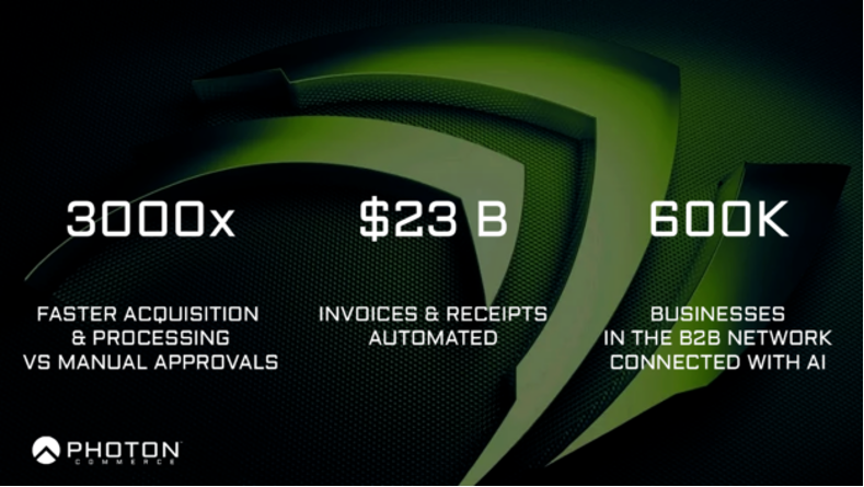
Partnering with NVIDIA and the ICC, Photon Commerce is creating the world’s most intelligent financial AI platform for instant B2B payments, invoices, statements, and receipts.
The business-to-business (B2B) payments ecosystem is massive, with $25 trillion in payments flowing between businesses each year. Photon Commerce, a financial AI platform company, empowers fintech leaders to process B2B payments, invoices, statements, and receipts instantly.
Over two-thirds of B2B transactions are processed through automated clearing house payments (a type of electronic payment) and checks. Yet, these transactions can take up to 3 days to clear. This has created a need for real-time payments that are processed instantaneously and safely, eliminating the risk of delinquent payments.
Partnering with NVIDIA and the International Chamber of Commerce, Photon Commerce guides payment processors, neobanks, and credit card fintechs on how to train and invent the world’s most intelligent AI for payments, invoices, and commerce.
Why is the use of AI crucial in payment processing? Card-not-present payments, such as those made online or over the phone, are costly for merchants, requiring manual entry and approval. AI-powered payments also work remotely but are instantaneous and secure.
Additionally, two out of three merchants today do not accept credit cards due to fees. Not even Amazon is willing to pay these expenses at times. The solution lies in real-time payments and request-for-payment offerings. These low-cost payment systems provide fraud-free payment options for 30 million merchants in the US.
Figure 1: Faster payment processing has led to the increased adoption of AI in the B2B sector.
One-click checkout for B2B transactions
Photon’s AI offers one-click bill pay for customers’ credit card lenders and leading core payment processors. These entities handle trillions of dollars in payments for the majority of banks and merchants.
One such customer, Settle is a leader in receivables finance, payables finance, and bill pay for eCommerce merchants like Italic, Huron, Brightland, and Branch.
Pioneering a Buy-Now-Pay-Later solution for B2B and eCommerce merchants, Settle Founder and CEO, Alek Koenig claims Photon’s invoice automation technology is a ‘godsend.’
“Photon’s solution enabled us to improve user experience, capture greater revenues, and significantly reduce manual keying of invoice and payment data. Before Photon, we were just typing up each invoice manually,” said Koenig.
Settle’s AI-based financial services and solutions achieved meteoric growth, especially among small to midsized businesses. The company raised nearly $100M from top-tier investors, such as Kleiner Perkins, within only 2 years of its inception.
55x the performance over CPUs
AI accelerated processing forms the underpinning of Photon Commerce’s AI solution capable of tackling unstructured or semistructured data and serving their customers. Photon’s base models for enterprise workloads start with 16 NVIDIA V100 GPUs. Depending on throughput, bandwidth, and power factors, Photon’s deep learning machines readily scale to 64 NVIDIA V100 GPUs or more.
GPU-accelerated computing has been critical to Photon’s machine learning models, both for training and inference. Photon’s deep learning was trained on NVIDIA V100s, providing 55x faster performance than CPU servers and 24x faster performance during inference.
Custom development and production boxes or clusters are provisioned either in the cloud, hybrid cloud, or on-prem deployments. Docker containers use Kubernetes to provide container orchestration across clusters during the scaling of models. Photon’s API architecture runs through a data pipeline of file validation, document classification, computer vision, then NLP. Photon’s NLP transformer models are autoregressive in architecture, employing model and data parallelism.
Next generation payment systems using AI
AI payment solution concepts are key to enabling end-to-end traceability, visibility, and scaling to high-transaction volumes needed for eCommerce merchants, and logistics companies for trade finance solutions.
Below are three examples of Photon’s AI solutions improving payment systems.
Receipts and invoices are made easier with Computer Vision/NLP
The value of extracting information from documents, particularly in the context of finance, for unstructured and semistructured data is enormous. Companies and individuals can process invoices, receipts, and forms with little to no-human interaction, saving time and money. Photon Commerce’s AI technology solves this problem by automatically reading, understanding, approving, and paying any invoice using computer vision and NLP.
Creating global standards for payment, invoice, and trade finance documentation using AI
Business documents are messy and each company has different Enterprise resource planning systems, record portals, and formats. These systems often break down with disputes, errors, and fraud happening daily. Photon Commerce’s solutions standardize any invoice, bill, or payment document in the world, regardless of language or format. This facilitates instant approvals, payments, and straight-through-processing.
Worldwide trade partners can now speak the same language and collaborate
Businesses and trade partners can now speak the same language. Photon’s NLP understands that a “vendor”, “supplier”, “seller”, “beneficiary”, “merchant”, and “卖方” are generally synonyms, referring to the same “object” called as Named Entity Recognition. Photon’s reconciliation AI can instantly flip any purchase order into an invoice, or match purchase orders, invoices, receipts, remittances, shipping labels, bills-of-lading, proof-of-deliveries, and rate confirmations seamlessly together.
See AI in action
Reach out to nvidia@photoncommerce.com and learn more about how AI accelerates payments, invoicing, and trade collaboration between businesses.
I’m tuning the hyperparameters of a Tensorflow model in Google AI platform, but I have the following problem: For the evaluation metric I want to optimize, it seems like only the metric value at the end of the training is reported to the hyperparameter optimizer, instead of the best value achieved during training. Is it possible to create a metric, which will track the maximum value over the entire training?
Despite these successes, it is still more effective to use classical algorithms for studying quantum chemistry than the noisy quantum processors we have available today. However, when the laws of quantum mechanics are translated into programs that a classical computer can run, we often find that the amount of time or memory required scales very poorly with the size of the physical system to simulate.
Today, in collaboration with Dr. Joonho Lee and Professor David Reichmann at Colombia, we present the Nature publication “Unbiasing Fermionic Quantum Monte Carlo with a Quantum Computer”, where we propose and experimentally validate a new way of combining classical and quantum computation to study chemistry, which can replace a computationally-expensive subroutine in a powerful classical algorithm with a “cheaper”, noisy, calculation on a small quantum computer. To evaluate the performance of this hybrid quantum-classical approach, we applied this idea to perform the largest quantum computation of chemistry to date, using 16 qubits to study the forces experienced by two carbon atoms in a diamond crystal. Not only was this experiment four qubits larger than our earlier chemistry calculations on Sycamore, we were also able to use a more comprehensive description of the physics that fully incorporated the interactions between electrons.
A New Way of Combining Quantum and Classical Our starting point was to use a family of Monte Carlo techniques (projector Monte Carlo, more on that below) to give us a useful description of the lowest energy state of a quantum mechanical system (like the two carbon atoms in a crystal mentioned above). However, even just storing a good description of a quantum state (the “wavefunction”) on a classical computer can be prohibitively expensive, let alone calculating one.
Projector Monte Carlo methods provide a way around this difficulty. Instead of writing down a full description of the state, we design a set of rules for generating a large number of oversimplified descriptions of the state (for example, lists of where each electron might be in space) whose average is a good approximation to the real ground state. The “projector” in projector Monte Carlo refers to how we design these rules — by continuously trying to filter out the incorrect answers using a mathematical process called projection, similar to how a silhouette is a projection of a three-dimensional object onto a two-dimensional surface.
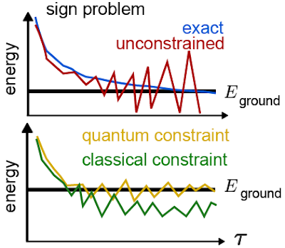
Unfortunately, when it comes to chemistry or materials science, this idea isn’t enough to find the ground state on its own. Electrons belong to a class of particles known as fermions, which have a surprising quantum mechanical quirk to their behavior. When two identical fermions swap places, the quantum mechanical wavefunction (the mathematical description that tells us everything there is to know about them) picks up a minus sign. This minus sign gives rise to the famous Pauli exclusion principle (the fact that two fermions cannot occupy the same state). It can also cause projector Monte Carlo calculations to become inefficient or even break down completely. The usual resolution to this fermionsign problem involves tweaking the Monte Carlo algorithm to include some information from an approximation to the ground state. By using an approximation (even a crude one) to the lowest energy state as a guide, it is usually possible to avoid breakdowns and even obtain accurate estimates of the properties of the true ground state.
Top: An illustration of how the fermion sign problem appears in some cases. Instead of following the blue line curve, our estimates of the energy follow the red curve and become unstable. Bottom: An example of the improvements we might see when we try to fix the sign problem. By using a quantum computer, we hope to improve the initial guess that guides our calculation and obtain a more accurate answer.
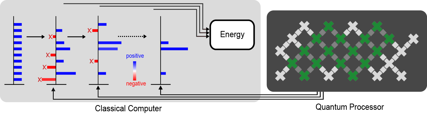
For the most challenging problems (such as modeling the breaking of chemical bonds), the computational cost of using an accurate enough initial guess on a classical computer can be too steep to afford, which led our collaborator Dr. Joonho Lee to ask if a quantum computer could help. We had already demonstrated in previous experiments that we can use our quantum computer to approximate the ground state of a quantum system. In these earlier experiments we aimed to measure quantities (such as the energy of the state) that are directly linked to physical properties (like the rate of a chemical reaction). In this new hybrid algorithm, we instead needed to make a very different kind of measurement: quantifying how far the states generated by the Monte Carlo algorithm on our classical computer are from those prepared on the quantum computer. Using some recently developed techniques, we were even able to do all of the measurements on the quantum computer before we ran the Monte Carlo algorithm, separating the quantum computer’s job from the classical computer’s.
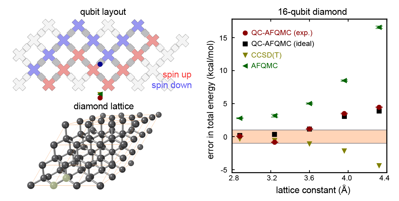
A diagram of our calculation. The quantum processor (right) measures information that guides the classical calculation (left). The crosses indicate the qubits, with the ones used for the largest experiment shaded green. The direction of the arrows indicate that the quantum processor doesn’t need any feedback from the classical calculation. The red bars represent the parts of the classical calculation that are filtered out by the data from the quantum computer in order to avoid the fermion sign problem and get a good estimate of properties like the energy of the ground state.
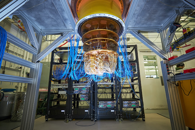
This division of labor between the classical and the quantum computer helped us make good use of both resources. Using our Sycamore quantum processor, we prepared a kind of approximation to the ground state that would be difficult to scale up classically. With a few hours of time on the quantum device, we extracted all of the data we needed to run the Monte Carlo algorithm on the classical computer. Even though the data was noisy (like all present-day quantum computations), it had enough signal that it was able to guide the classical computer towards a very accurate reconstruction of the true ground state (shown in the figure below). In fact, we showed that even when we used a low-resolution approximation to the ground state on the quantum computer (just a few qubits encoding the position of the electrons), the classical computer could efficiently solve a much higher resolution version (with more realism about where the electrons can be).
Top left: a diagram showing the sixteen qubits we used for our largest experiment. Bottom left: an illustration of the carbon atoms in a diamond crystal. Our calculation focused on two atoms (the two that are highlighted in translucent yellow). Right: A plot showing how the error in the total energy (closer to zero is better) changes as we adjust the lattice constant (the spacing between the two carbon atoms). Many properties we might care about, such as the structure of the crystal, can be determined by understanding how the energy varies as we move the atoms around. The calculations we performed using the quantum computer (red points) are comparable in accuracy to two state-of-the-art classical methods (yellow and green triangles) and are extremely close to the numbers we would have gotten if we had a perfect quantum computer rather than a noisy one (black points). The fact that these red and black points are so close tells us that the error in our calculation comes from using an approximate ground state on the quantum computer that was too simple, not from being overwhelmed by noise on the device.
Using our new hybrid quantum algorithm, we performed the largest ever quantum computation of chemistry or materials science. We used sixteen qubits to calculate the energy of two carbon atoms in a diamond crystal. This experiment was four qubits larger than our first chemistry calculations on Sycamore, we obtained more accurate results, and we were able to use a better model of the underlying physics. By guiding a powerful classical Monte Carlo calculation using data from our quantum computer, we performed these calculations in a way that was naturally robust to noise.
We’re optimistic about the promise of this new research direction and excited to tackle the challenge of scaling these kinds of calculations up towards the boundary of what we can do with classical computing, and even to the hard-to-study corners of the universe. We know the road ahead of us is long, but we’re excited to have another tool in our growing toolbox.
Acknowledgements I’d like to thank my co-authors on the manuscript, Bryan O’Gorman, Nicholas Rubin, David Reichman, Ryan Babbush, and especially Joonho Lee for their many contributions, as well as Charles Neill and Pedram Rousham for their help executing the experiment. I’d also like to thank the larger Google Quantum AI team, who designed, built, programmed, and calibrated the Sycamore processor.
I wanted to do a group project on tensorflow object detection for university, but, our teacher wanted us to use our own images instead of datasets. The project is a road safety app that can detect and label road signs, oncoming vehicles and pedestrians. Is this going to be too much to handle , is it possible to make a app that can detect these things using custom images or is it impossible?
(Side note : i can also reduce the project to just detection and recognition of road signs and vehicles)
Posted by Arsha Nagrani and Chen Sun, Research Scientists, Google Research, Perception Team
People interact with the world through multiple sensory streams (e.g., we see objects, hear sounds, read words, feel textures and taste flavors), combining information and forming associations between senses. As real-world data consists of various signals that co-occur, such as video frames and audio tracks, web images and their captions and instructional videos and speech transcripts, it is natural to apply a similar logic when building and designing multimodal machine learning (ML) models.
Effective multimodal models have wide applications — such as multilingual image retrieval, future action prediction, and vision-language navigation — and are important for several reasons; robustness, which is the ability to perform even when one or more modalities is missing or corrupted, and complementarity between modalities, which is the idea that some information may be present only in one modality (e.g., audio stream) and not in the other (e.g., video frames). While the dominant paradigm for multimodal fusion, called late fusion, consists of using separate models to encode each modality, and then simply combining their output representations at the final step, investigating how to effectively and efficiently combine information from different modalities is still understudied.
In “Attention Bottlenecks for Multimodal Fusion”, published at NeurIPS 2021, we introduce a novel transformer-based model for multimodal fusion in video called Multimodal BottleneckTransformer (MBT). Our model restricts cross-modalattention flow between latent units in two ways: (1) through tight fusion bottlenecks, that force the model to collect and condense the most relevant inputs in each modality (sharing only necessary information with other modalities), and (2) to later layers of the model, allowing early layers to specialize to information from individual modalities. We demonstrate that this approach achieves state-of-the-art results on video classification tasks, with a 50% reduction in FLOPs compared to a vanilla multimodal transformer model. We have also released our code as a tool for researchers to leverage as they expand on multimodal fusion work.
A Vanilla Multimodal Transformer Model Transformer models consistently obtain state-of-the-art results in ML tasks, including video (ViViT) and audio classification (AST). Both ViViT and AST are built on the Vision Transformer (ViT); in contrast to standard convolutional approaches that process images pixel-by-pixel, ViT treats an image as a sequence of patch tokens (i.e., tokens from a smaller part, or patch, of an image that is made up of multiple pixels). These models then perform self-attention operations across all pairs of patch tokens. However, using transformers for multimodal fusion is challenging because of their high computational cost, with complexity scaling quadratically with input sequence length.
Because transformers effectively process variable length sequences, the simplest way to extend a unimodal transformer, such as ViT, to the multimodal case is to feed the model a sequence of both visual and auditory tokens, with minimal changes to the transformer architecture. We call this a vanilla multimodal transformer model, which allows free attention flow (called vanilla cross-attention) between different spatial and temporal regions in an image, and across frequency and time in audio inputs, represented by spectrograms. However, while easy to implement by concatenating audio and video input tokens, vanilla cross-attention at all layers of the transformer model is unnecessary because audio and visual inputs contain dense, fine-grained information, which may be redundant for the task — increasing complexity.
Restricting Attention Flow The issue of growing complexity for long sequences in multimodal models can be mitigated by reducing the attention flow. We restrict attention flow using two methods, specifying the fusion layer and addingattention bottlenecks.
Fusion layer (early, mid or late fusion): In multimodal models, the layer where cross-modal interactions are introduced is called the fusion layer. The two extreme versions are early fusion (where all layers in the transformer are cross-modal) and late fusion (where all layers are unimodal and no cross-modal information is exchanged in the transformer encoder). Specifying a fusion layer in between leads to mid fusion. This technique builds on a common paradigm in multimodal learning, which is to restrict cross-modal flow to later layers of the network, allowing early layers to specialize in learning and extracting unimodal patterns.
Attention bottlenecks: We also introduce a small set of latent units that form an attention bottleneck (shown below in purple), which force the model, within a given layer, to collate and condense information from each modality before sharing it with the other, while still allowing free attention flow within a modality. We demonstrate that this bottlenecked version (MBT), outperforms or matches its unrestricted counterpart with lower computational cost.
The different attention configurations in our model. Unlike late fusion (top left), where no cross-modal information is exchanged in the transformer encoder, we investigate two pathways for the exchange of cross-modal information. Early and mid fusion (top middle, top right) is done via standard pairwise self attention across all hidden units in a layer. For mid fusion, cross-modal attention is applied only to later layers in the model. Bottleneck fusion (bottom left) restricts attention flow within a layer through tight latent units called attention bottlenecks. Bottleneck mid fusion (bottom right) applies both forms of restriction in conjunction for optimal performance.
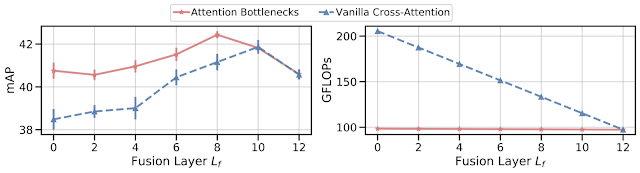
Bottlenecks and Computation Cost We apply MBT to the task of sound classification using the AudioSet dataset and investigate its performance for two approaches: (1) vanilla cross-attention, and (2) bottleneck fusion. For both approaches, mid fusion (shown by the middle values of the x-axis below) outperforms both early (fusion layer = 0) and late fusion (fusion layer = 12). This suggests that the model benefits from restricting cross-modal connections to later layers, allowing earlier layers to specialize in learning unimodal features; however, it still benefits from multiple layers of cross-modal information flow. We find that adding attention bottlenecks (bottleneck fusion) outperforms or maintains performance with vanilla cross-attention for all fusion layers, with more prominent improvements at lower fusion layers.
The impact of using attention bottlenecks for fusion on mAP performance (left) and compute (right) at different fusion layers on AudioSet. Attention bottlenecks (red) improve performance over vanilla cross-attention (blue) at lower computational cost. Mid fusion, which is in fusion layers 4-10, outperforms both early (fusion layer = 0) and late (fusion layer = 12) fusion, with best performance at fusion layer 8.
We compare the amount of computation, measured in GFLOPs, for both vanilla cross-attention and bottleneck fusion. Using a small number of attention bottlenecks (four bottleneck tokens used in our experiments) adds negligible extra computation over a late fusion model, with computation remaining largely constant with varying fusion layers. This is in contrast to vanilla cross-attention, which has a non-negligible computational cost for every layer it is applied to. We note that for early fusion, bottleneck fusion outperforms vanilla cross-attention by over 2 mean average precision points (mAP) on audiovisual sound classification, with less than half the computational cost.
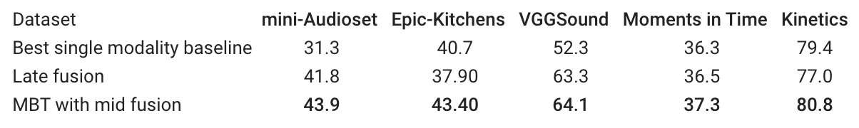
Results on Sound Classification and Action Recognition MBT outperforms previous research on popular video classification tasks — sound classification (AudioSet and VGGSound) and action recognition (Kinetics and Epic-Kitchens). For multiple datasets, late fusion and MBT with mid fusion (both fusing audio and vision) outperform the best single modality baseline, and MBT with mid fusion outperforms late fusion.
Across multiple datasets, fusing audio and vision outperforms the best single modality baseline, and MBT with mid fusion outperforms late fusion. For each dataset we report the widely used primary metric, i.e., Audioset: mAP, Epic-Kitchens: Top-1 action accuracy, VGGSound, Moments-in-Time and Kinetics: Top-1 classification accuracy.
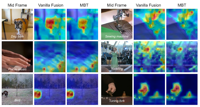
Visualization of Attention Heatmaps To understand the behavior of MBT, we visualize the attention computed by our network following the attention rollout technique. We compute heat maps of the attention from the output classification tokens to the image input space for a vanilla cross-attention model and MBT on the AudioSet test set. For each video clip, we show the original middle frame on the left with the ground truth labels overlayed at the bottom. We demonstrate that the attention is particularly focused on regions in the images that contain motion and create sound, e.g., the fingertips on the piano, the sewing machine, and the face of the dog. The fusion bottlenecks in MBT further force the attention to be localized to smaller regions of the images, e.g., the mouth of the dog in the top left and the woman singing in the middle right. This provides some evidence that the tight bottlenecks force MBT to focus only on the image patches that are relevant for an audio classification task and that benefit from mid fusion with audio.
Summary We introduce MBT, a new transformer-based architecture for multimodal fusion, and explore various fusion approaches using cross-attention between bottleneck tokens. We demonstrate that restricting cross-modal attention via a small set of fusion bottlenecks achieves state-of-the-art results on a number of video classification benchmarks while also reducing computational costs compared to vanilla cross-attention models.
Acknowledgements This research was conducted by Arsha Nagrani, Anurag Arnab, Shan Yang, Aren Jansen, Cordelia Schmid and Chen Sun. The blog post was written by Arsha Nagrani, Anurag Arnab and Chen Sun. Animations were created by Tom Small.

 Partnering with NVIDIA and the ICC, Photon Commerce is creating the world’s most intelligent financial AI platform for instant B2B payments, invoices, statements, and receipts.