Categories
Offsites

GraphWorld: Advances in Graph Benchmarking

Graphs are very common representations of natural systems that have connected relational components, such as social networks, traffic infrastructure, molecules, and the internet. Graph neural networks (GNNs) are powerful machine learning (ML) models for graphs that leverage their inherent connections to incorporate context into predictions about items within the graph or the graph as a whole. GNNs have been effectively used to discover new drugs, help mathematicians prove theorems, detect misinformation, and improve the accuracy of arrival time predictions in Google Maps.

A surge of interest in GNNs during the last decade has produced thousands of GNN variants, with hundreds introduced each year. In contrast, methods and datasets for evaluating GNNs have received far less attention. Many GNN papers re-use the same 5–10 benchmark datasets, most of which are constructed from easily labeled academic citation networks and molecular datasets. This means that the empirical performance of new GNN variants can be claimed only for a limited class of graphs. Confounding this issue are recently published works with rigorous experimental designs that cast doubt on the performance rankings of popular GNN models reported in seminal papers.

Recent workshops and conference tracks devoted to GNN benchmarking have begun addressing these issues. The recently-introduced Open Graph Benchmark (OGB) is an open-source package for benchmarking GNNs on a handful of massive-scale graph datasets across a variety of tasks, facilitating consistent GNN experimental design. However, the OGB datasets are sourced from many of the same domains as existing datasets, such as citation and molecular networks. This means that OGB does not solve the dataset variety problem we mention above. Therefore, we ask: how can the GNN research community keep up with innovation by experimenting on graphs with the large statistical variance seen in the real-world?

To match the scale and pace of GNN research, in “GraphWorld: Fake Graphs Bring Real Insights for GNNs”, we introduce a methodology for analyzing the performance of GNN architectures on millions of synthetic benchmark datasets. Whereas GNN benchmark datasets featured in academic literature are just individual “locations” on a fully-diverse “world” of potential graphs, GraphWorld directly generates this world using probability models, tests GNN models at every location on it, and extracts generalizable insights from the results. We propose GraphWorld as a complementary GNN benchmark that allows researchers to explore GNN performance on regions of graph space that are not covered by popular academic datasets. Furthermore, GraphWorld is cost-effective, running hundreds-of-thousands of GNN experiments on synthetic data with less computational cost than one experiment on a large OGB dataset.

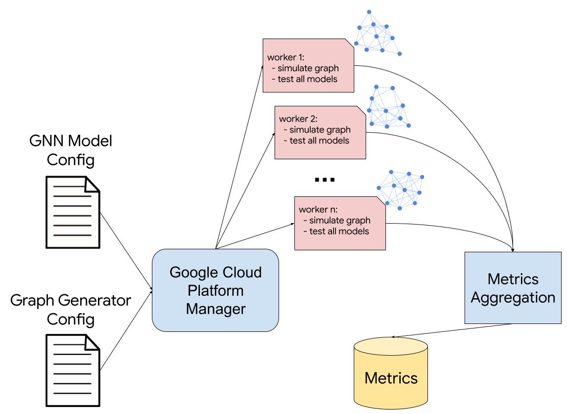
Illustration of the GraphWorld pipeline. The user provides configurations for the graph generator and the GNN models to test. GraphWorld spawns workers, each one simulating a new graph with diverse properties and testing all specified GNN models. The test metrics from the workers are then aggregated and stored for the user.

The Limited Variety of GNN Benchmark Datasets
To illustrate the motivation for GraphWorld, we compare OGB graphs to a much larger collection (5,000+) of graphs from the Network Repository. While the vast majority of Network Repository graphs are unlabelled, and therefore cannot be used in common GNN experiments, they represent a large space of graphs that are available in the real world. We computed two properties of the OGB and Network Repository graphs: the clustering coefficient (how interconnected nodes are to nearby neighbors) and the degree distribution gini coefficient (the inequality among the nodes’ connection counts). We found that OGB datasets exist in a limited and sparsely-populated region of this metric space.

The distribution of graphs from the Open Graph Benchmark does not match the larger population of graphs from the Network Repository.

Dataset Generators in GraphWorld
A researcher using GraphWorld to investigate GNN performance on a given task first chooses a parameterized generator (example below) that can produce graph datasets for stress-testing GNN models on the task. A generator parameter is an input that controls high-level features of the output dataset. GraphWorld uses parameterized generators to produce populations of graph datasets that are varied enough to test the limits of state-of-the-art GNN models.

For instance, a popular task for GNNs is node classification, in which a GNN is trained to infer node labels that represent some unknown property of each node, such as user interests in a social network. In our paper, we chose the well-known stochastic block model (SBM) to generate datasets for this task. The SBM first organizes a pre-set number of nodes into groups or “clusters“, which serve as node labels to be classified. It then generates connections between nodes according to various parameters that (each) control a different property of the resulting graph.

One SBM parameter that we expose to GraphWorld is the “homophily” of the clusters, which controls the likelihood that two nodes from the same cluster are connected (relative to two nodes from different clusters). Homophily is a common phenomenon in social networks in which users with similar interests (e.g., the SBM clusters) are more likely to connect. However, not all social networks have the same level of homophily. GraphWorld uses the SBM to generate graphs with high homophily (below on the left), graphs with low homophily (below on the right), and millions more graphs with any level of homophily in-between. This allows a user to analyze GNN performance on graphs with all levels of homophily without depending on the availability of real-world datasets curated by other researchers.
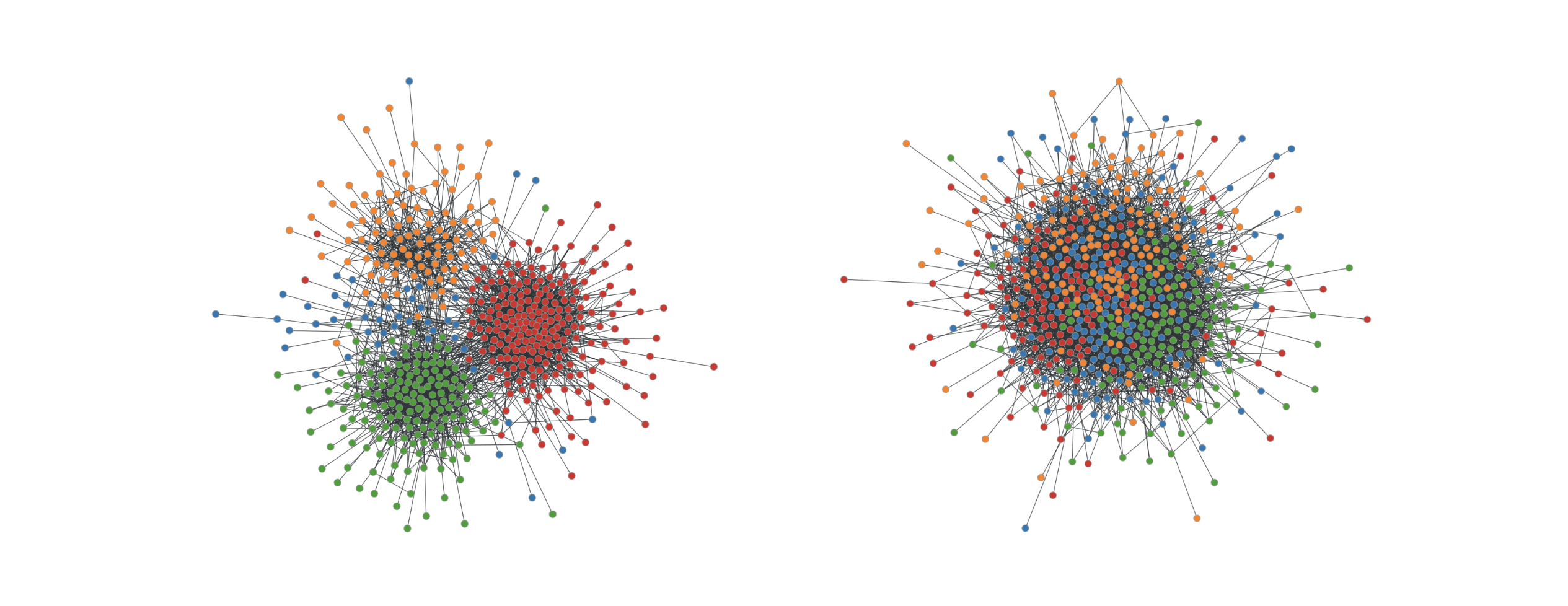
Examples of graphs produced by GraphWorld using the stochastic block model. The left graph has high homophily among node classes (represented by different colors); the right graph has low homophily.

GraphWorld Experiments and Insights
Given a task and parameterized generator for that task, GraphWorld uses parallel computing (e.g., Google Cloud Platform Dataflow) to produce a world of GNN benchmark datasets by sampling the generator parameter values. Simultaneously, GraphWorld tests an arbitrary list of GNN models (chosen by the user, e.g., GCN, GAT, GraphSAGE) on each dataset, and then outputs a massive tabular dataset joining graph properties with the GNN performance results.

In our paper, we describe GraphWorld pipelines for node classification, link prediction, and graph classification tasks, each featuring different dataset generators. We found that each pipeline took less time and computational resources than state-of-the-art experiments on OGB graphs, which means that GraphWorld is accessible to researchers with low budgets.

The animation below visualizes GNN performance data from the GraphWorld node classification pipeline (using the SBM as the dataset generator). To illustrate the impact of GraphWorld, we first map classic academic graph datasets to an xy plane that measures the cluster homophily (x-axis) and the average of the node degrees (y-axis) within each graph (similar to the scatterplot above that includes the OGB datasets, but with different measurements). Then, we map each simulated graph dataset from GraphWorld to the same plane, and add a third z-axis that measures GNN model performance over each dataset. Specifically, for a particular GNN model (like GCN or GAT), the z-axis measures the mean reciprocal rank of the model against the 13 other GNN models evaluated in our paper, where a value closer to 1 means the model is closer to being the top performer in terms of node classification accuracy.

The animation illustrates two related conclusions. First, GraphWorld generates regions of graph datasets that extend well-beyond the regions covered by the standard datasets. Second, and most importantly, the rankings of GNN models change when graphs become dissimilar from academic benchmark graphs. Specifically, the homophily of classic datasets like Cora and CiteSeer are high, meaning that nodes are well-separated in the graph according to their classes. We find that as GNNs traverse toward the space of less-homophilous graphs, their rankings change quickly. For example, the comparative mean reciprocal rank of GCN moves from higher (green) values in the academic benchmark region to lower (red) values away from that region. This shows that GraphWorld has the potential to reveal critical headroom in GNN architecture development that would be invisible with only the handful of individual datasets that academic benchmarks provide.

Relative performance results of three GNN variants (GCN, APPNP, FiLM) across 50,000 distinct node classification datasets. We find that academic GNN benchmark datasets exist in GraphWorld regions where model rankings do not change. GraphWorld can discover previously unexplored graphs that reveal new insights about GNN architectures.

Conclusion
GraphWorld breaks new ground in GNN experimentation by allowing researchers to scalably test new models on a high-dimensional surface of graph datasets. This allows fine-grained analysis of GNN architectures against graph properties on entire subspaces of graphs that are distal from Cora-like graphs and those in the OGB, which appear only as individual points in a GraphWorld dataset. A key feature of GraphWorld is its low cost, which enables individual researchers without access to institutional resources to quickly understand the empirical performance of new models.

With GraphWorld, researchers can also investigate novel random/generative graph models for more-nuanced GNN experimentation, and potentially use GraphWorld datasets for GNN pre-training. We look forward to supporting these lines of inquiry with our open-source GraphWorld repository and follow-up projects.

Acknowledgements
GraphWorld is joint work with Brandon Mayer and Bryan Perozzi from Google Research. Thanks to Tom Small for visualizations.

Categories
Misc

Upcoming Event:  Accelerating the Creation of Custom, Production-Ready AI Models for Edge AI

Visit NVIDIA in booth 806 at the Embedded Vision Summit 2022 and join a session to learn how the NVIDIA TAO Toolkit can help you create custom AI models without AI expertise.

Categories
Misc

Five Features for Enhancing Your Workspace with NVIDIA RTX Software

Learn how you can make the most out of graphics workflows with NVIDIA RTX Desktop Manager and NVIDIA RTX Experience.
From digital content creation to product design, graphics workflows are becoming more complex, interactive, and collaborative. As many organizations around the world adjust to a hybrid work environment, designers, engineers, developers, and other professionals are constantly setting up workspaces that best suit them, no matter where they are working from.

Users can easily create optimal settings to customize their workspace and enhance productivity and efficiency with NVIDIA RTX software. 

NNVIDIA RTX software has two offerings aimed at enhancing productivity:

  • NVIDIA RTX Desktop Manager: users can manage single or multi-display workspaces with ease, providing maximum flexibility and control over display real estate and desktops. 
  • NVIDIA RTX Experience: delivers productivity tools such as driver management and content capture, to minimize context-switching over GPU tools so users can focus on their work.  

Check out the top five features of NVIDIA RTX Desktop Manager and RTX Experience.

Instant, automatic downloads

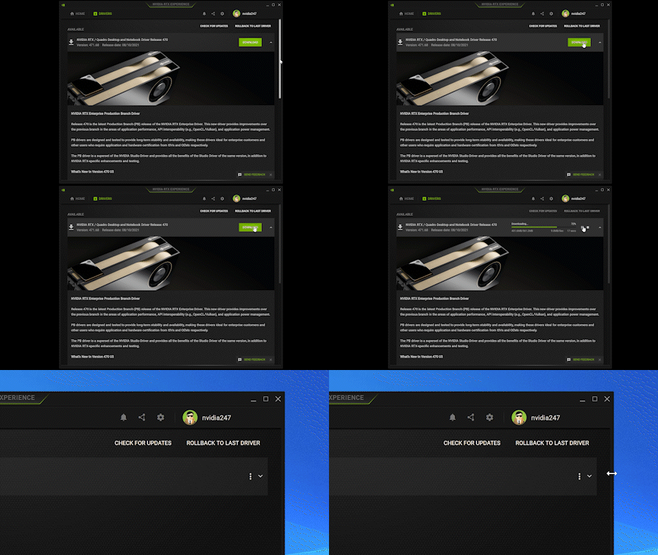
Get automatic alerts from NVIDIA RTX Experience whenever a new driver is available. Instantly download and install the drivers from the application, shaving multiple steps from the normal download and install process. And if you need something from the previous driver, the rollback feature provides easy reinstallation.

Animation of driver install and rollback in RTX Experience.
Figure 1. Install new drivers or rollback to previous ones with NVIDIA RTX Experience.

Desktop recording on demand

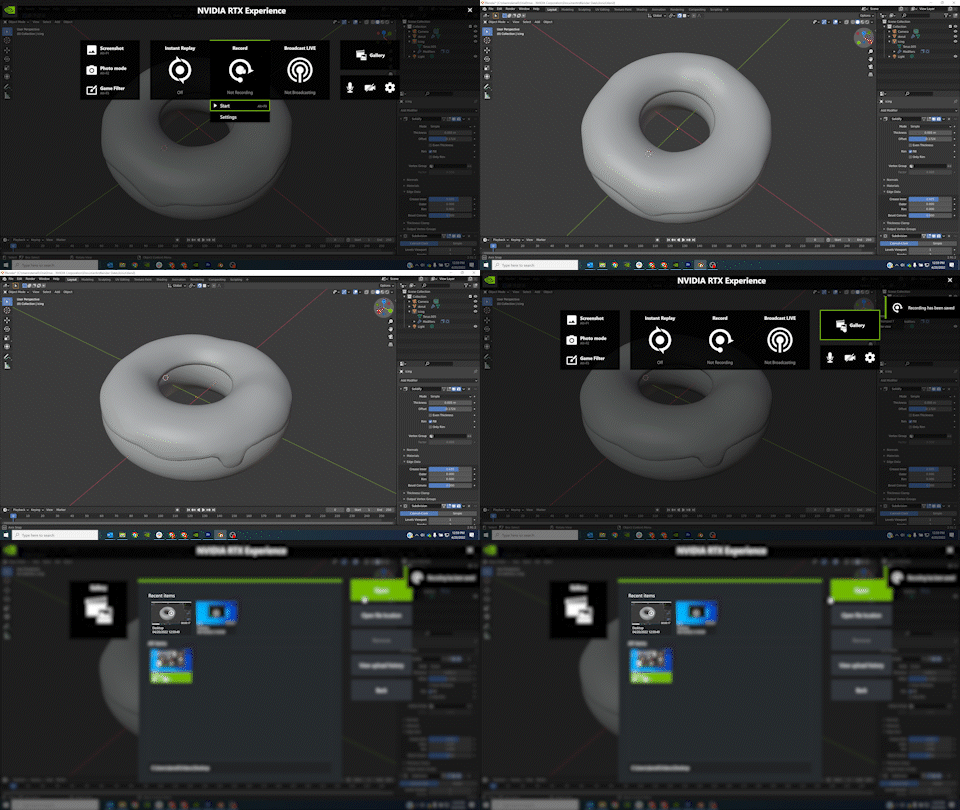
Use NVIDIA RTX Experience hotkeys to start recording your desktop instantly to capture images or create how-to videos to share with others. Recordings are automatically saved in a convenient repository for easy access. This is great for troubleshooting, as well.

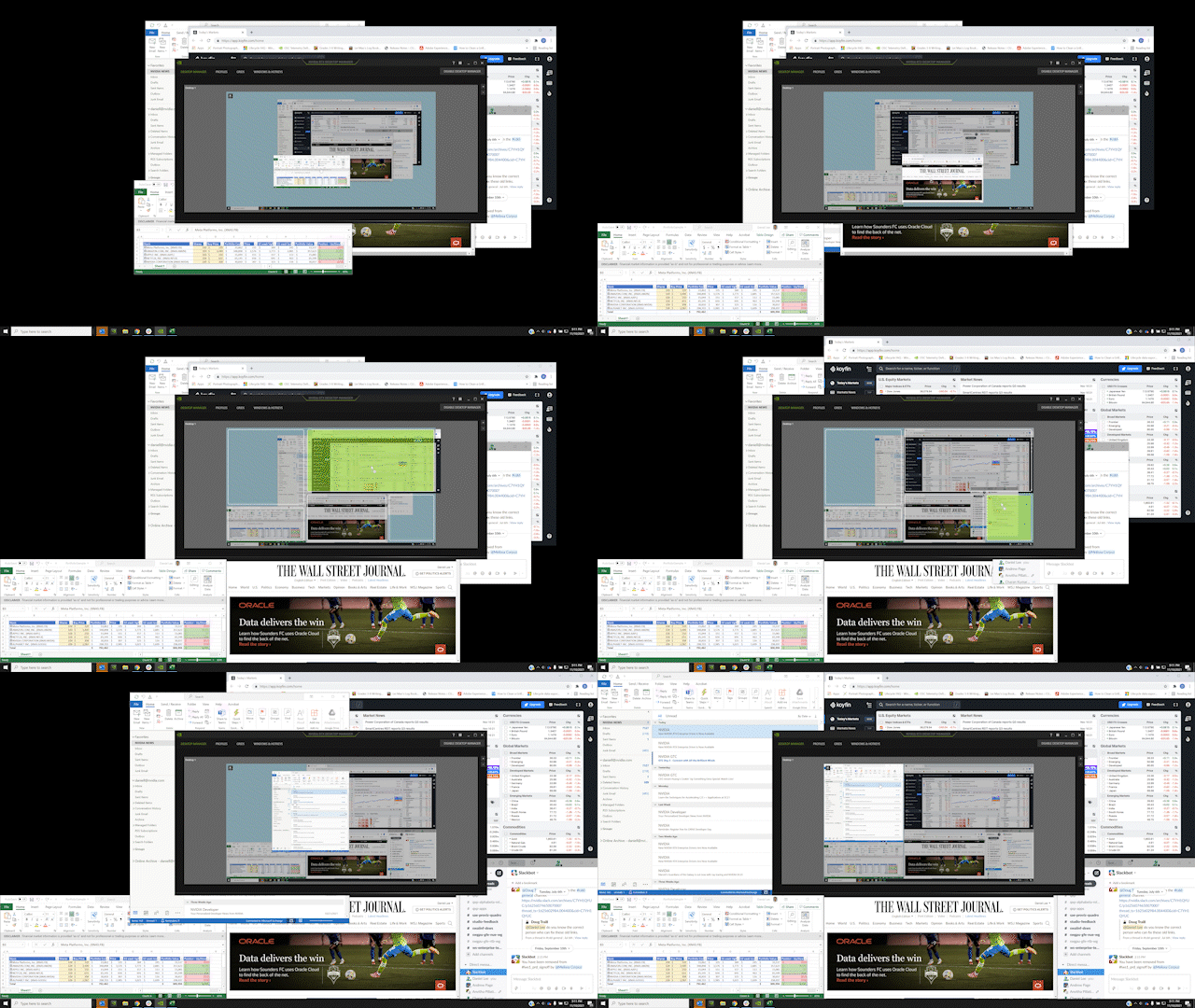
Sequence showing 3D model sequence being captured by RTX Experience.
Figure 2. Use hotkeys to start recording your screen instantly.

Snap Windows to grids

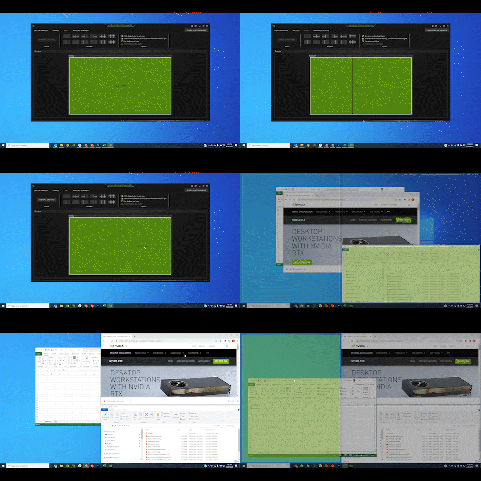
Use NVIDIA RTX Desktop Manager to snap windows quickly into predefined grids, and change grid configurations easily to suit specific workflows or projects. This will help maximize display real estate—while staying in tune with your aesthetics.

Graphic shows grids on the desktop, and multiple windows being snapped to each grid.
Figure 3. Quickly snap windows into custom grids with NVIDIA RTX Desktop Manager.

See everything from a bird’s-eye view


Manage all of your physical and virtual desktops from within the RTX Desktop Manager’s Birdseye View interface. No need to scroll or drag windows across monitors to organize and snap things into place—do it all from one central location.

Animation of screen shows multiple windows open and dragged around the desktop.
Figure 4. Manage all your windows within the RTX Desktop Manager Birdseye View interface.

Maximize productivity with layers


Having trouble finding that app buried beneath other windows? Use the RTX Desktop Manager’s expanded toolset to toggle desired apps to ‘Always Remain on Top of the Desktop.’ You can also set the transparency level of that top window to see what is going on underneath. This is also a great trick for taking notes while on a video call.

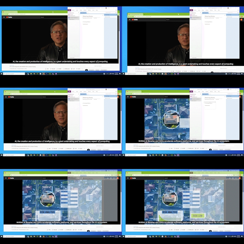
Image shows a video playing in the background while a notes application is at the forefront at various transparency levels.
Figure 5. Set specific windows to remain on top of other applications, as well as transparency levels.

NVIDIA RTX software is available to all users who have RTX GPUs.

Download NVIDIA RTX Desktop Manager and NVIDIA RTX Experience today, and get the productivity tools to enhance work from anywhere.

Categories
Misc

Setting AIs on SIGGRAPH: Top Academic Researchers Collaborate With NVIDIA to Tackle Graphics’ Greatest Challenges

NVIDIA’s latest academic collaborations in graphics research have produced a reinforcement learning model that smoothly simulates athletic moves, ultra-thin holographic glasses for virtual reality, and a real-time rendering technique for objects illuminated by hidden light sources. These projects — and over a dozen more — will be on display at SIGGRAPH 2022, taking place Aug. Read article >

The post Setting AIs on SIGGRAPH: Top Academic Researchers Collaborate With NVIDIA to Tackle Graphics’ Greatest Challenges appeared first on NVIDIA Blog.

Categories
Misc

New on NGC: One Click Deploy, AI Models for Speech and Computer Vision, and More

This month the NGC catalog added a new one-click deploy feature, new speech and computer vision models, and sample speech training data to help simplify your AI app development.
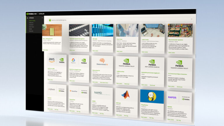
The NVIDIA NGC catalog is a hub for GPU-optimized deep learning, machine learning, and HPC applications. With highly performant software containers, pretrained models, industry-specific SDKs, and Jupyter Notebooks the content helps simplify and accelerate end-to-end workflows. 

New features, software, and updates to help you streamline your workflow and build your solutions faster on NGC include:

One Click Deploy

Developing AI with your favorite tool, Jupyter Notebooks, just got easier with simplified software deployment using the NGC catalog’s new one-click deploy feature.

Simply go to the software page in the NGC catalog and click on “Deploy to Vertex AI” to get started. Under the hood, this feature: launches the JupyterLab instance on Google Cloud Vertex AI Workbench with optimal configuration; preloads the software dependencies; and downloads the NGC notebook in one go. You can also change the configuration before launching the instance.

Release highlights:

  • Jupyter Notebooks for popular AI use-cases.
  • One Click Deploy runs NGC Jupyter Notebooks on a Google Cloud Vertex AI Workbench.
  • Automated setup with optimal configuration, preloaded dependencies, and ready-to-run notebooks.
  • Data scientists can focus on building production-grade models for faster time to market.

See the collection of AI software and Notebooks that you can deploy with one click.

Register for our upcoming webinar to learn how you can use our new feature to build and run your machine learning app 5X faster.

NVIDIA Virtual Machine Image

Virtual Machine Image (VMI) or AMI (in case of AWS) are like operating systems that run on top of the hypervisor on cloud platforms.

NVIDIA GPU-optimized VMI provides a standardized image across IaaS platforms so developers develop their AI application once, whether on NVIDIA-Certified Systems or any GPU cloud instance, and deploy the application on any cloud without code change.

Figure 1. NVIDIA VMI provides a standardized stack across clouds for organizations to deploy their applications anywhere without code change.

Available from the respective cloud marketplaces, the NVIDIA VMIs are tested on NVIDIA AI software from the NGC catalog to deliver optimized performance and are updated quarterly with the latest drivers, security patches, and support for the latest GPUs.

Organizations may purchase enterprise support of NVIDIA AI software so developers can outsource technical issues and instead focus on building and running AI.

Build your AI today with NVIDIA VMI on AWS, Azure, and Google Cloud.

Deep learning software

The most popular deep learning frameworks for training and inference are updated monthly. Pull the latest version (v22.04) of:

New speech and computer vision models

We are constantly adding state-of-the-art models for a variety of speech and vision models. Here is a list of a handful of new models. 

  • STT Hi Conformer: Transcribes speech in Hindi characters along with spaces.
  • Riva Conformer ASR Spanish: Transcribes speech in lowercase Spanish alphabet.
  • EfficientNet v2-S: A family of image classification models, which achieve state-of-the-art accuracy, being an order-of magnitude smaller and faster.
  • GatorTron-S: A Megatron BERT model trained on synthetic clinical discharge summaries.
  • BioMegatron345m: This NeMo model delivers improved results on a range of biomedical downstream tasks.

To explore more models, visit the NGC Models page.

Sample speech training data

To help you customize pretrained models for your speech application, Defined.AI, an NVIDIA partner, is offering 30 minutes of free sample data for eight languages.

Access it now through the NGC catalog.

HPC Applications

The latest versions of popular HPC applications are also available in the NGC catalog including:

  • HPC SDK: A comprehensive suite of compilers, libraries, and HPC tools.
  • MATLAB: Provides algorithms, pretrained models, and apps to create, train, visualize, and optimize deep neural networks.

Visit the NGC catalog to see how the GPU-optimized software can help simplify workflows and speed up solution times.

Categories
Misc

Hello, beginner requiring help here

I’ve just picked up tensorflow and I’m trying to make a simple Siamese neural network.

How would I import csv’s as the left and right input? Any help would be greatly appreciated

def siamese_model(input_shape):

“””

Model Architecture

“””

# define the tensor for the two input texts

left_input = Input(input_shape1)

right_input = Input(input_shape2)

# convolutional neural network

model = Sequential()

model.add(Conv2D(64, (10,10),activation=’relu’,input_shape=input_shape,

kernel_initializer=initialize_weights, kernal_regularizer=12(2e-4)))

model.add(MaxPooling2D())

model.add(Conv2D(128, (7,7),activation=’relu’,

kernel_initializer=initialize_weights,

bias_initializer=initialize_bias, kernel_regularizer=12(2e-4)))

model.add(MaxPooling2D())

model.add(Conv2D(128, (4,4),activation=’relu’,

kernel_initializer=initialize_weights,

bias_initializer=initialize_bias, kernel_regularizer=12(2e-4)))

model.add(MaxPooling2D())

model.add(Conv2D(256, (4,4),activation=’relu’,

kernel_initializer=initialize_weights,

bias_initializer=initialize_bias, kernel_regularizer=12(2e-4)))

model.add(Flatten())

model.add(Dense(4096,activation=’sigmoid’,

kernel_regularizer=12(1e-3),

kernel_initializer=initialize_weights,bias_initializer=bias_initializer))

# Generate the encodings (feature vectors) for the two images

encoded_l = model(left_input)

encoded_r = model(right_input)

# Add a custom layer to compute the absolute difference between the encodings

l1_layer = Lambda(lambda tensors:K.abs(tensors[0] – tensors[1]))

l1_distance = l1_layer([encoded_l, encoded_r])

# Add a denselayer with a sigmoid unit to generate the similarity score

prediction = Dense(1,activation=’sigmoid’,bias_initializer=initialize_bias)(l1_distance)

#connect the inputs with the outputs

siamese_net = Model(inputs=[left_input, right_input],outputs=prediction)

# return model

return siamese_netamese_net

submitted by /u/Issue_647
[visit reddit] [comments]

Categories
Misc

Problem with Tensorflow cast function and the GPU

I am trying to normalize a numpy array with tf.cast(array, tf.float32)/255.0.

When I run the script I am running into an error:

Traceback (most recent call last):

, line 91, in normalize

normalized = tf.cast(array, tf.float32) / 255.0

, line 153, in error_handler

raise e.with_traceback(filtered_tb) from None

site-packagestensorflowpythonframeworkops.py”, line 7186, in raise_from_not_ok_status

raise core._status_to_exception(e) from None # pylint: disable=protected-access

tensorflow.python.framework.errors_impl.ResourceExhaustedError: failed to allocate memory [Op:Cast]

submitted by /u/Successful-Ad-8021
[visit reddit] [comments]

Categories
Misc

How to see the CNN layer result?

Hi, I’m experimenting with CNN and I want to know if there’s a way to extract the output of a CNN layer and plot as an image to see what pattern my network identify in that layer.

submitted by /u/Current_Falcon_3187
[visit reddit] [comments]

Categories
Misc

Numpy to tfRecord

What is the best way to convert dataset from numpy to tfRecord? I try going through tensorflow documentation, it just make think worse.

submitted by /u/InternalStorm133
[visit reddit] [comments]

Categories
Offsites

Alpa: Automated Model-Parallel Deep Learning

Over the last several years, the rapidly growing size of deep learning models has quickly exceeded the memory capacity of single accelerators. Earlier models like BERT (with a parameter size of < 1GB) can efficiently scale across accelerators by leveraging data parallelism in which model weights are duplicated across accelerators while only partitioning and distributing the training data. However, recent large models like GPT-3 (with a parameter size of 175GB) can only scale using model parallel training, where a single model is partitioned across different devices.

While model parallelism strategies make it possible to train large models, they are more complex in that they need to be specifically designed for target neural networks and compute clusters. For example, Megatron-LM uses a model parallelism strategy to split the weight matrices by rows or columns and then synchronizes results among devices. Device placement or pipeline parallelism partitions different operators in a neural network into multiple groups and the input data into micro-batches that are executed in a pipelined fashion. Model parallelism often requires significant effort from system experts to identify an optimal parallelism plan for a specific model. But doing so is too onerous for most machine learning (ML) researchers whose primary focus is to run a model and for whom the model’s performance becomes a secondary priority. As such, there remains an opportunity to automate model parallelism so that it can easily be applied to large models.

In “Alpa: Automating Inter- and Intra-Operator Parallelism for Distributed Deep Learning”, published at OSDI 2022, we describe a method for automating the complex model parallelism process. We demonstrate that with only one line of code Alpa can transform any JAX neural network into a distributed version with an optimal parallelization strategy that can be executed on a user-provided device cluster. We are also excited to release Alpa’s code to the broader research community.

Alpa Design
We begin by grouping existing ML parallelization strategies into two categories, inter-operator parallelism and intra-operator parallelism. Inter-operator parallelism assigns distinct operators to different devices (e.g., device placement) that are often accelerated with a pipeline execution schedule (e.g., pipeline parallelism). With intra-operator parallelism, which includes data parallelism (e.g., Deepspeed-Zero), operator parallelism (e.g., Megatron-LM), and expert parallelism (e.g., GShard-MoE), individual operators are split and executed on multiple devices, and often collective communication is used to synchronize the results across devices.

The difference between these two approaches maps naturally to the heterogeneity of a typical compute cluster. Inter-operator parallelism has lower communication bandwidth requirements because it is only transmitting activations between operators on different accelerators. But, it suffers from device underutilization because of its pipeline data dependency, i.e., some operators are inactive while waiting on the outputs from other operators. In contrast, intra-operator parallelism doesn’t have the data dependency issue, but requires heavier communication across devices. In a GPU cluster, the GPUs within a node have higher communication bandwidth that can accommodate intra-operator parallelism. However, GPUs across different nodes are often connected with much lower bandwidth (e.g., ethernet) so inter-operator parallelism is preferred.

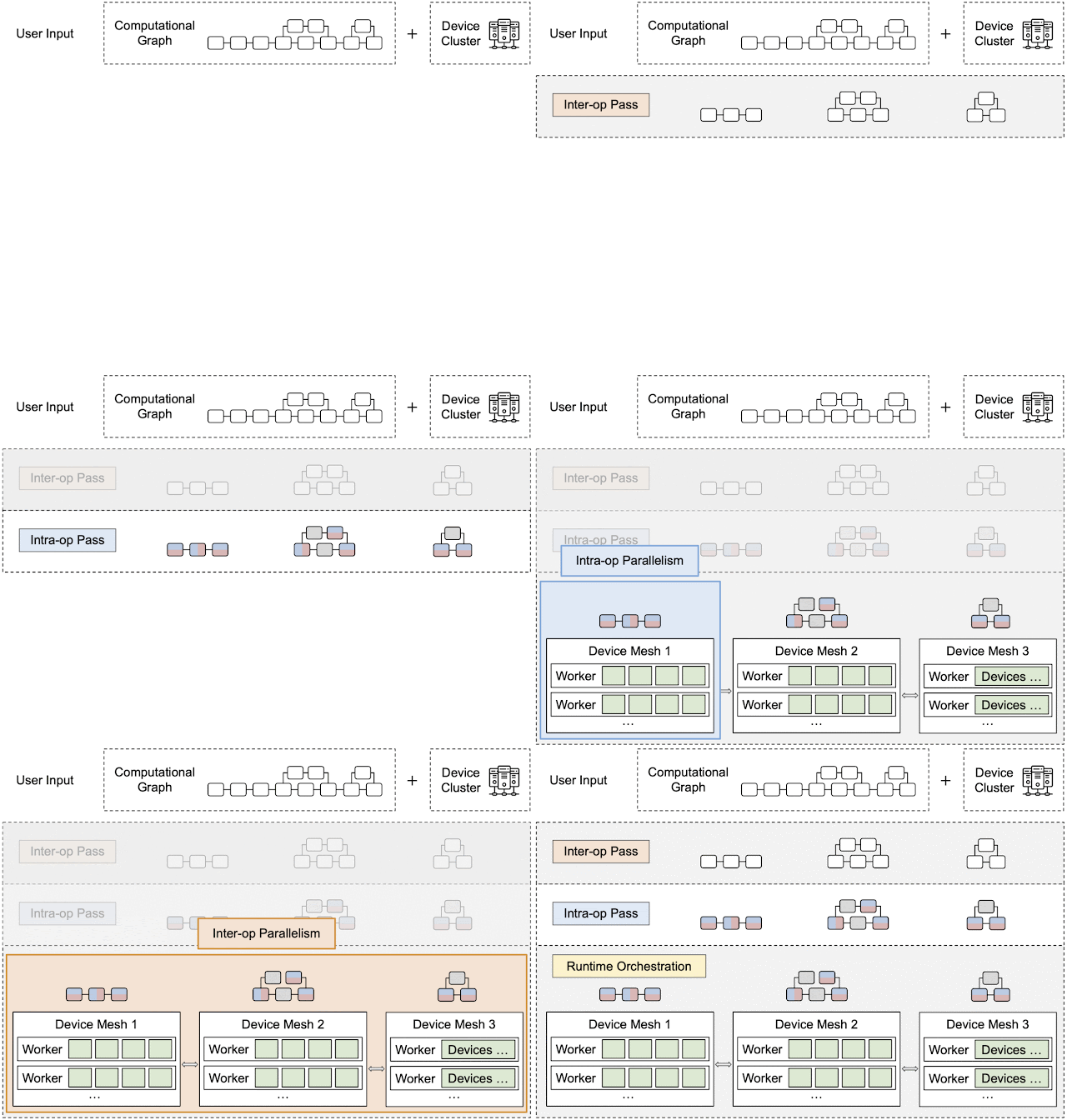
By leveraging heterogeneous mapping, we design Alpa as a compiler that conducts various passes when given a computational graph and a device cluster from a user. First, the inter-operator pass slices the computational graph into subgraphs and the device cluster into submeshes (i.e., a partitioned device cluster) and identifies the best way to assign a subgraph to a submesh. Then, the intra-operator pass finds the best intra-operator parallelism plan for each pipeline stage from the inter-operator pass. Finally, the runtime orchestration pass generates a static plan that orders the computation and communication and executes the distributed computational graph on the actual device cluster.

An overview of Alpa. In the sliced subgraphs, red and blue represent the way the operators are partitioned and gray represents operators that are replicated. Green represents the actual devices (e.g., GPUs).

Intra-Operator Pass
Similar to previous research (e.g., Mesh-TensorFlow and GSPMD), intra-operator parallelism partitions a tensor on a device mesh. This is shown below for a typical 3D tensor in a Transformer model with a given batch, sequence, and hidden dimensions. The batch dimension is partitioned along device mesh dimension 0 (mesh0), the hidden dimension is partitioned along mesh dimension 1 (mesh1), and the sequence dimension is replicated to each processor.

A 3D tensor that is partitioned on a 2D device mesh.

With the partitions of tensors in Alpa, we further define a set of parallelization strategies for each individual operator in a computational graph. We show example parallelization strategies for matrix multiplication in the figure below. Defining parallelization strategies on operators leads to possible conflicts on the partitions of tensors because one tensor can be both the output of one operator and the input of another. In this case, re-partition is needed between the two operators, which incurs additional communication costs.

The parallelization strategies for matrix multiplication.

Given the partitions of each operator and re-partition costs, we formulate the intra-operator pass as a Integer-Linear Programming (ILP) problem. For each operator, we define a one-hot variable vector to enumerate the partition strategies. The ILP objective is to minimize the sum of compute and communication cost (node cost) and re-partition communication cost (edge cost). The solution of the ILP translates to one specific way to partition the original computational graph.

Inter-Operator Pass
The inter-operator pass slices the computational graph and device cluster for pipeline parallelism. As shown below, the boxes represent micro-batches of input and the pipeline stages represent a submesh executing a subgraph. The horizontal dimension represents time and shows the pipeline stage at which a micro-batch is executed. The goal of the inter-operator pass is to minimize the total execution latency, which is the sum of the entire workload execution on the device as illustrated in the figure below. Alpa uses a Dynamic Programming (DP) algorithm to minimize the total latency. The computational graph is first flattened, and then fed to the intra-operator pass where the performance of all possible partitions of the device cluster into submeshes are profiled.

Pipeline parallelism. For a given time, this figure shows the micro-batches (colored boxes) that a partitioned device cluster and a sliced computational graph (e.g., stage 1, 2, 3) is processing.

Runtime Orchestration
After the inter- and intra-operator parallelization strategies are complete, the runtime generates and dispatches a static sequence of execution instructions for each device submesh. These instructions include RUN a specific subgraph, SEND/RECEIVE tensors from other meshes, or DELETE a specific tensor to free the memory. The devices can execute the computational graph without other coordination by following the instructions.

Evaluation
We test Alpa with eight AWS p3.16xlarge instances, each of which has eight 16 GB V100 GPUs, for 64 total GPUs. We examine weak scaling results of growing the model size while increasing the number of GPUs. We evaluate three models: (1) the standard Transformer model (GPT); (2) the GShard-MoE model, a transformer with mixture-of-expert layers; and (3) Wide-ResNet, a significantly different model with no existing expert-designed model parallelization strategy. The performance is measured by peta-floating point operations per second (PFLOPS) achieved on the cluster.

We demonstrate that for GPT, Alpa outputs a parallelization strategy very similar to the one computed by the best existing framework, Megatron-ML, and matches its performance. For GShard-MoE, Alpa outperforms the best expert-designed baseline on GPU (i.e., Deepspeed) by up to 8x. Results for Wide-ResNet show that Alpa can generate the optimal parallelization strategy for models that have not been studied by experts. We also show the linear scaling numbers for reference.

GPT: Alpa matches the performance of Megatron-ML, the best expert-designed framework.
GShard MoE: Alpa outperforms Deepspeed (the best expert-designed framework on GPU) by up to 8x.
Wide-ResNet: Alpa generalizes to models without manual plans. Pipeline and Data Parallelism (PP-DP) is a baseline model that uses only pipeline and data parallelism but no other intra-operator parallelism.
The parallelization strategy for Wide-ResNet on 16 GPUs consists of three pipeline stages and is a complicated strategy even for an expert to design. Stages 1 and 2 are on 4 GPUs performing data parallelism, and stage 3 is on 8 GPUs performing operator parallelism.

Conclusion
The process of designing an effective parallelization plan for distributed model-parallel deep learning has historically been a difficult and labor-intensive task. Alpa is a new framework that leverages intra- and inter-operator parallelism for automated model-parallel distributed training. We believe that Alpa will democratize distributed model-parallel learning and accelerate the development of large deep learning models. Explore the open-source code and learn more about Alpa in our paper.

Acknowledgements
Thanks to the co-authors of the paper: Lianmin Zheng, Hao Zhang, Yonghao Zhuang, Yida Wang, Danyang Zhuo, Joseph E. Gonzalez, and Ion Stoica. We would also like to thank Shibo Wang, Jinliang Wei, Yanping Huang, Yuanzhong Xu, Zhifeng Chen, Claire Cui, Naveen Kumar, Yash Katariya, Laurent El Shafey, Qiao Zhang, Yonghui Wu, Marcello Maggioni, Mingyao Yang, Michael Isard, Skye Wanderman-Milne, and David Majnemer for their collaborations to this research.