We currently have a decent machine learning pipeline going on but new projects/demands are coming and we’re now lacking coputational power to run everything in time. Since hardware prices skyrocketed since the begining of this pandemic, a local upgrade would be very expensive, so we’re looking for alternatives.
Can anyone suggest and comment your experience with some of these cloud GPU services? We’re running trainings 24/7 on our local machines and more “horsepower” would be appreciated. We’re looking into Paperspace Gradient, but it seems a bit of an overkill (but still cheap) and AWS.
As one can see the results (0.2 and -1.17) are completely different. Same saved_model was used in all cases.
Note: TF-serving is run under docker-compose and the service “tf-serving” is using the official tensorflow/serving image
I would appreciate any hits and testing suggestions.
If there are better solutions to run multiple TF models in production than TF-serving (except Cloud-based solutions like SageMaker) please share some knowledge with me.
Notes:
Batching is disabled by default settings, but I disabled it manually too
There are 4 different models that produce different type of output (single value, set of values, bitmap data). ALL 4 have different result while being served by TFServing and plain TF. Dimensions of the output tensors are fine, values they have are “wrong”.
cuFFTMp is a multi-node, multi-process extension to cuFFT that enables scientists and engineers to solve challenging problems on exascale platforms.
Today, NVIDIA announces the release of cuFFTMp for Early Access (EA). cuFFTMp is a multi-node, multi-process extension to cuFFT that enables scientists and engineers to solve challenging problems on exascale platforms.
FFTs (Fast Fourier Transforms) are widely used in a variety of fields, ranging from molecular dynamics, signal processing, computational fluid dynamics (CFD) to wireless multimedia and machine learning applications. With cuFFTMp, NVIDIA now supports not only multiple GPUs within a single system, but many GPUs across multiple nodes.
Figure 1 shows cuFFTMp reaching over 1.8 PFlop/s, more than 70% of the peak machine bandwidth for a transform of that scale.
Figure 1. cuFFTMp (weak scaling) performances on the Selene cluster
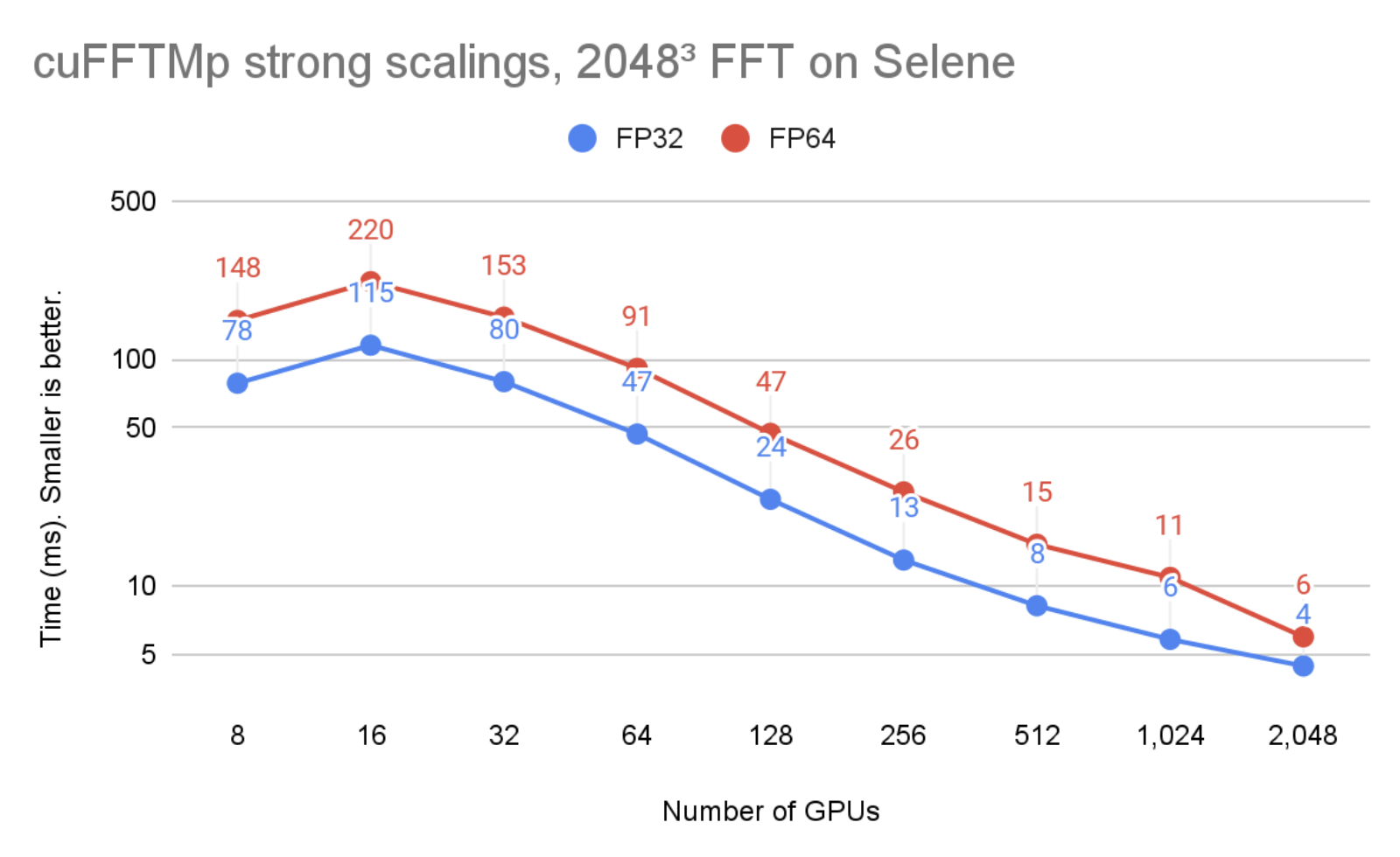
In Figure 2, the problem size is kept unchanged but the number of GPUs is increased from 8 to 2048. You can see that cuFFTMp successfully strong-scales the problem, bringing the single-precision time from 78ms with 8 GPUs (1 node) to 4ms with 2048 GPUs (256 nodes).
Figure 2. cuFFTMp (strong scaling) performances on the Selene cluster
Figure 1 and 2 were run on the Selene cluster. Selene is made of NVIDIA DGXA100, 8xA100-80GB per node with NVSwitch (300 GB/s/GPU, bidirectional) and Mellanox Infiniband HDR (200 GB/s/node, bidirectional). Tests were ran using CUDA 11.4 and the NVIDIA HPC SDK 21.9 Docker container, available at nvcr.io/nvidia/nvhpc:21.9-runtime-cuda11.4-ubuntu20.04. GPU application clocks were set to the maximum.
Performance and scalability
Distributed 3D FFTs are well-known to be communication-bound because of global collective communications of the MPI_Alltoallv type. MPI_Alltoallv is the main bottleneck for distributed FFTs due to low internode bandwidth relative to high compute capabilities, and accelerator-aware MPI implementations of all_to_all type of communications vary in quality.
cuFFTMp uses NVSHMEM, a new communication library based on the OpenSHMEM standard and designed for NVIDIA GPUs by providing kernel-initiated communications. NVSHMEM creates a global address space that includes the memory of all GPUs in the cluster. Performing communication from inside CUDA kernels enables fine-grained, remote data access that reduces synchronization cost and takes advantage of the massive parallelism in the GPU to hide communication overheads.
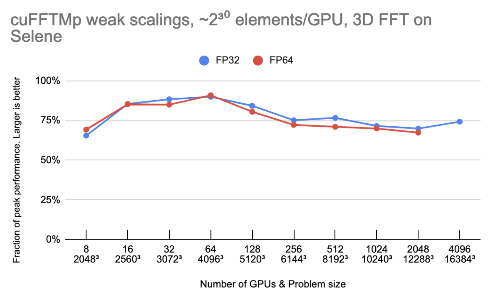
Figure 3 shows that cuFFTMp is able to maintain roughly 75% peak as the number of GPUs are doubled.
Figure 3. Weak scalings of cuFFTMp on the Selene cluster, displayed as a fraction of the peak performances
Peak performance is using 2000 GB/s/gpu for bidirectional global memory bandwidth, 300 GB/s/gpu for bidirectional NVLink bandwidth and 25 GB/s/gpu for Infiniband bandwidth.
Let N be the 1D transform size and G the number of GPUs. Every GPU owns N3/G elements (8 or 16 bytes each), and the model assumes that N3/G elements are read/written six times to or from global memory and N3/G2 elements are sent one time from every GPU to every other GPU. On 4096 GPUs, the time spent in non-InfiniBand communications accounts for less than 10% of the total time.
MPI portability and multi-architecture support
As mentioned earlier, the performances of cuFFTMp do not depend on the MPI implementation. For portability, cuFFTMp requires MPI to be launched and to manage data distributions on the CPUs.
Currently cuFFTMp statically links to NVSHMEM. NVSHMEM uses a small MPI “bootstrap plugin” (nvshmem_bootstrap_mpi.so), which is built using MPI and automatically loaded at runtime. This bootstrap targets the OpenMPI version included in the HPC SDK. For user applications that depend on another MPI implementation, the EA package includes helper scripts to build a bootstrap targeting a different MPI.
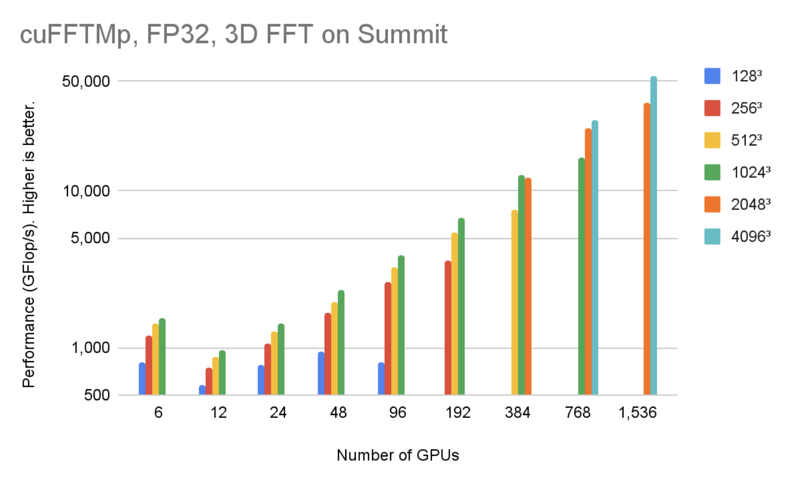
cuFFTMp supports both Linux x86_64 and IBM POWER architecture. You can download the EA package for different architectures. Figure 4 shows that, using 1536 V100 GPUs in 256 nodes, cuFFTMp can reach over 50 TFlop/s transforming 40963 complex data points with only 5% of the Summit system.
Figure 4. cuFFTMp (FP32) performances on the Summit cluster
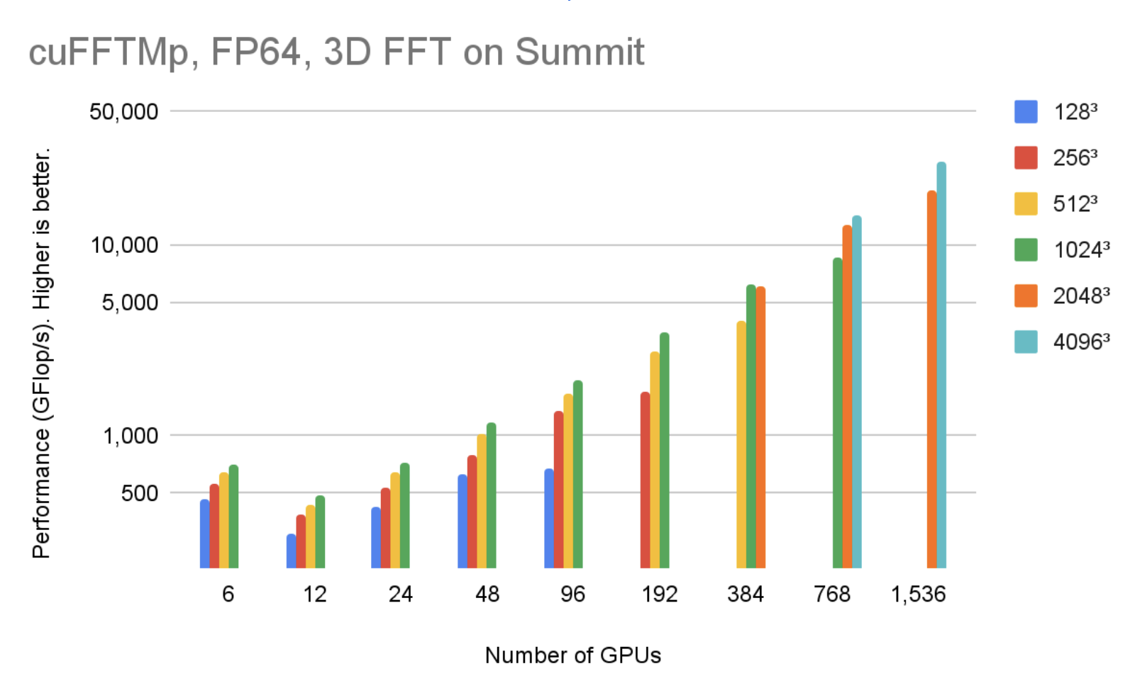
Figure 5 shows that, using 1536 V100 GPUs in 256 nodes, cuFFTMp can reach over 40 TFlop/s transforming 40963 complex data points with only 5% of the Summit system.
Figure 5. cuFFTMp (FP64) performances on the Summit cluster
Easy transition to cuFFTMp
cuFFTMp is simply an extension to the current multi-GPU cuFFT library. Most existing multi-GPU functions apply to cuFFTMp. As a distributed, multiprocess library, cuFFTMp requires MPI to be bootstrapped (“launched”) and expects that data is distributed among MPI processes. The following table shows the code required to convert an application from using multi-GPU cuFFT to cuFFTMp.
Multi-GPU, single-process cuFFT
cuFFTMp
#include
#include #include
MPI_Init(&argc, &argv); int rank, size; MPI_Comm_rank(MPI_COMM_WORLD, &rank); MPI_Comm_size(MPI_COMM_WORLD, &size); cudaSetDevice(my_device);
size_t my_NX = (NX / size) + (rank size ? 1 : 0);
// host buffer h_f size NX*NY*NZ
// host buffer h_f size my_NX*NY*NZ
cufftHandle plan_c2c; cufftCreate(&plan_c2c);
for (auto i = 0; i whichGPUs[i] = i; cufftXtSetGPUs(plan_c2c, NGPUS, whichGPUs)
Slab, pencil, and block decompositions are typical names of data distribution methods in multidimensional FFT algorithms for the purposes of parallelizing the computation across nodes. cuFFTMp EA only supports optimized slab (1D) decompositions, and provides helper functions, for example cufftXtSetDistribution and cufftMpReshape, to help users redistribute from any other data distributions to cuFFTMp’s slab data distribution.
The cuFFTMp EA package includes C++ and Fortran samples that cover a range of use cases: C2C, R2C/C2R, different plans sharing workspace, and shuffling data from one distribution to the other or redistributing across GPUs. cuFFTMp provides full support for Fortran applications, using the HPC SDK 21.7+ compilers and wrappers included in the EA package.
To understand turbulence flow behavior, a research team at the Tata Institute of Fundamental Research-Hyderabad India (TFRI) developed Fluid3D, a CFD package applying direct numerical simulation (DNS) of the Navier-Stokes equations with pseudo-spectral methods. By porting Fluid3D to cuFFTMp and CUDA, the team can now simulate higher Reynolds number flow on thousands of GPUs within a few hours, an impossible task using the MPI CPU version.
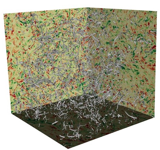
In Figure 6, turbulent flows consist of vortices of different scales, and energy is transferred from larger scales of motion to the small scales. It is important to simulate and understand the isotropic behavior of the smallest turbulent structures in large DNS runs.
Figure 6. DNS turbulence flow simulation using Fluid3D
DNS is a key tool to improve the understanding of turbulence flows, and pseudo-spectral methods are commonly used because of their computational efficiency and accuracy.
The challenge of turbulence flow simulation is the need to attain high Reynolds (Re) numbers. To maintain the computational stability, the Re number is limited by the grid resolution, that is, Re2.25N3, where N is the number of grid points in each dimension. Therefore, simulating high Re number turbulence flows requires numerical resolutions that can be computationally costly or even prohibitive.
Table 1 shows the grid resolutions required for the maximum Re numbers and the memory requirements for the simulations.
Grid resolution
Simulated Reynolds number
Memory requirement (GB)
10243
199.2
88
20483
316.2
704
40963
501.9
5,632
81923
796.8
45,056
122883
1044.1
152,064
163843
1264.8
360,448
Table 1. The Turbulence DNS package Fluid3D requires large numerical resolution and system memory to simulate high Reynolds number flow
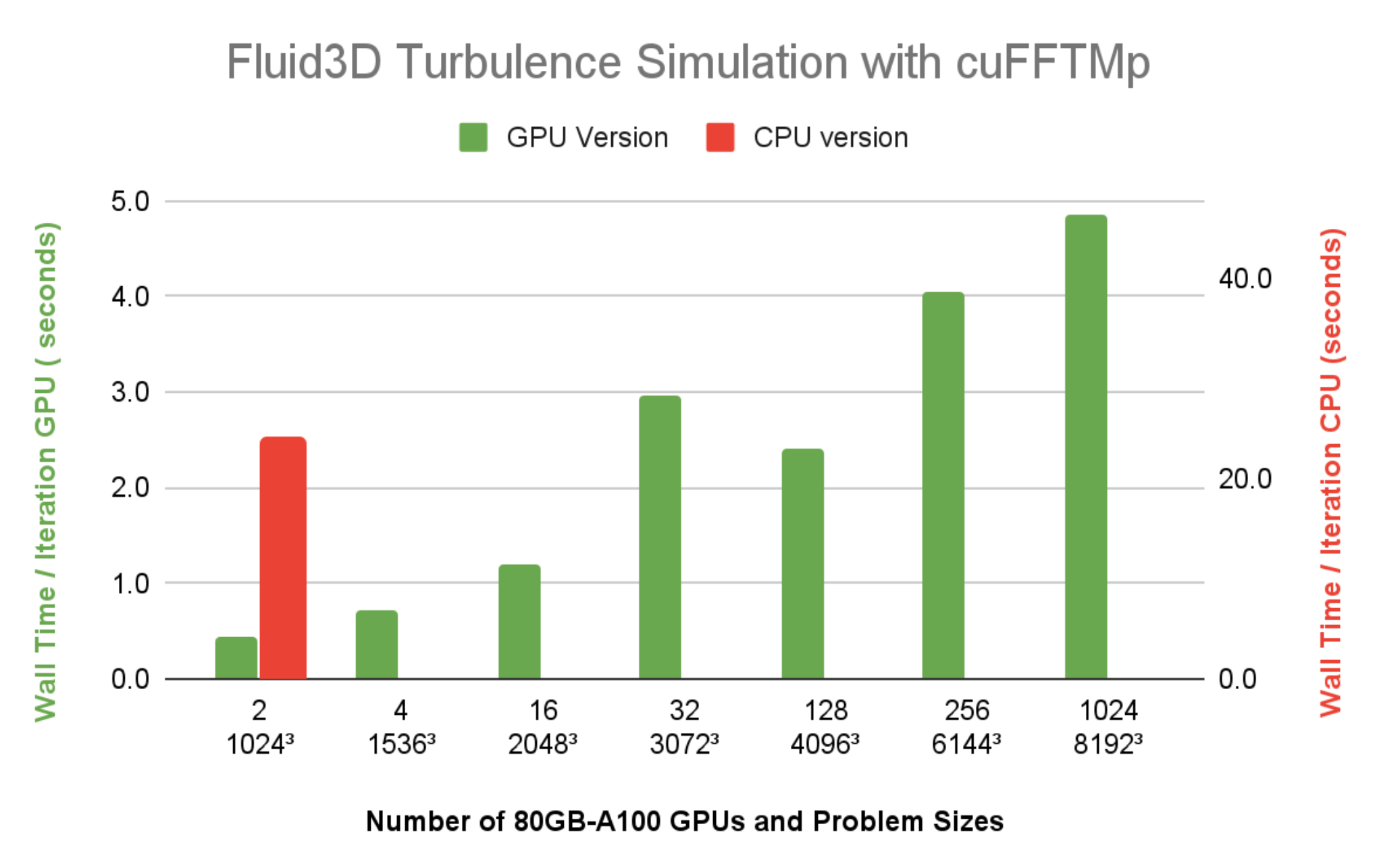
Fluid3D uses a second-order exponential Adams-Bashforth time-stepping method in the Fourier space. The simulations are typically integrated over tens of thousands of time steps, computing nine 3D-FFTs per time step. FFTs dominate the overall simulation runtime. The elapsed wall time per time step is an important metric to gauge whether the time to solution for a particular configuration of numerical experiment is reasonable.
Figure 7 shows the wall time per time step of Fluid3D is under 5 seconds, at a resolution of 81923, using 1024 A100 GPUs (128 nodes) on Selene. The CPU version with FFTW-MPI, takes 23.9 seconds per time iteration, for a resolution of 10243 problem size using 64 MPI ranks on a single 64-core CPU node. Compared to the wall time running the same 10243 problem size using two A100 GPUs, it’s clear that the speedup of Fluid3D from a CPU node to a single A100 is more than 20x.
Figure 7. Wall time per time step of Fluid3D DNS running on Selene
Get started with cuFFTMp
Interested in trying out cuFFTMp to transition your application to run on multiple nodes? Head over to the Getting Started page of cuFFTMp EA. After downloading cuFFTMp, play with the sample code and see how similar they are to the multi-GPU version and how they can scale over multiple nodes.
We continue working on improving cuFFTMp, including adding batched APIs, as well as data compression to minimize communications. If you have questions or new feature requests, contact product manager Matthew Nicely.
Acknowledgments
Special thanks to Prasad Perlekar’s team at Tata Institute of Fundamental Research in Hyderabad, India, for giving us access to the multiphase turbulence flow code Fluid3D and becoming the first adopter of cuFFTMp.
We also thank the entire NVSHMEM team at NVIDIA for their help supporting the development of cuFFTMp.
Nsight Compute kernel profiler now includes Range Replay, Memory Analysis, and Guided Analysis enhancements.
NVIDIA Nsight Compute is an interactive kernel profiler for CUDA applications. It provides detailed performance metrics and API debugging through a user interface and a command-line tool. Nsight Compute 2022.1 brings updates to improve data collection modes enabling new use cases and options for performance profiling.
This release of Nsight Compute extends the existing replay modes with the highly requested feature of Range Replay. Range Replay captures and replays complete ranges of CUDA API calls and kernel launches within the profiled application. Metrics are associated with the entire range as opposed to individual kernels.This allows the tool to execute kernels without serialization and support profiling kernels that need to be run concurrently for correctness or performance reasons. A range consists of a start and an end marker; and includes all CUDA API calls and kernels launched between these markers from any CPU thread.
Figure 1. Visualization of Range Replay: After capturing the range, each pass collects performance information for the entire range.
Memory Analysis
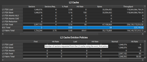
When profiling on A100, a new L2 Cache Eviction Policies table in the Memory Analysis section helps you understand the number of accesses and achieved hit rates by the various cache eviction policies. In the same section, the L2 Cache table now has a new ECC row to show traffic created from enabling hardware Error Correction Code on the GPU.
Figure 2. Improvements to the Memory Workload Analysis tables: ECC and L2 cache eviction policy information.
Guided Analysis
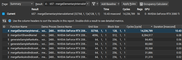
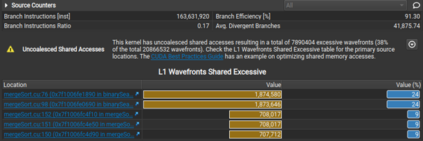
Nsight Compute now makes it easier to select initial analysis targets in multiresult collection by dynamically selecting between the Summary and Details pages when opening a report. Rules were extended to detect non-fused floating-point instructions as an optimization opportunity. Last, but not least, when the Uncoalesced Memory Access rules are triggered, they show a table of the five most valuable instances, making it easier to inspect and resolve them on the Source page.
Figure 3. Opening multiresult reports now shows the Summary page, allowing you to sort results and decide on the optimization order.
Figure 4. Both Uncoalesced Memory Access rules present results in a more concise and sorted format.
Additional improvements
Further improvements include an Occupancy Calculator auto-update. There is also a new ‘Thread Instructions Executed’ metric and register name tooltips for the Register Dependency columns in the Source page, as well as NVLink updates.
At GTC in November of 2021, we released insightful assets showcasing Nsight tools capabilities:
With NVIDIA Jetson embedded platforms, teams at the DARPA SubT Challenge detected objects with both high accuracy and high throughput.
Performing real-time inference with high accuracy is a challenging task, especially in a poor-visibility environment. With NVIDIA Jetson embedded platforms, teams at the recently concluded Defense Advanced Research Projects Agency (DARPA) Subterranean (SubT) Challenge were able to detect objects of interest with both high accuracy and high throughput. In this post, we will cover the results, systems, and challenges faced by teams in the final leg of the systems competition.
The SubT Challenge is an international robotics competition organized and coordinated by DARPA. The competition encourages researchers to develop new approaches for robots to map, navigate, and search environments that pose various challenges such as poor visibility, presence of hazards, unknown maps, or poor communication infrastructure.
The challenge consists of three preliminary circuit events: Tunnel Circuit, Urban Circuit, and Cave Circuit (canceled due to the COVID-19 pandemic), as well as a final integrated challenge course. Each circuit and the final event are held in different environments with various types of terrain. According to the event organizers, the competition was held over 3 years in different phases with the final event held in September of 2021 in Louisville, KY.
Competitors in the SubT Challenge leveraged NVIDIA technology for both their hardware and software needs. Teams used desktop/server GPUs to train models that were deployed on robots using NVIDIA Jetson embedded platform for real-time detection of artifacts and objects of interest–the main criteria used to determine the winning team. Five out of seven competitors also used the Jetson platform to perform real-time object detection.
The SubT Challenge
The SubT Challenge is inspired by real-world scenarios faced by first responders during search and rescue operations or disaster response.
The state-of-the-art methods developed through this competition will help reduce the risk of casualties of search and rescue personnel and first responders while they explore the unknown underground environments. Additionally, the autonomous robots will assist personnel in exploring the environment to find survivors, objects of interest, and access locations that are otherwise risky for humans.
Figure 1. The DARPA Subterranean Challenge explores innovative approaches and new technologies to map, navigate, and search complex underground environments. — Image courtesy of DARPA.
Technical challenges
The competition incorporates various technical challenges such as dealing with unknown, unstructured, and uneven terrain that some robots might not be able to maneuver easily.
These environments typically would not have any infrastructure for communication with the central command. From a perception perspective, these environments will have poor visibility where the robots must find artifacts and objects of interest.
The competing teams were tasked with addressing these challenges by developing novel sensor fusion methods as well as developing new or modifying existing robotic platforms with different capabilities to locate and detect objects of interest.
Team CERBERUS
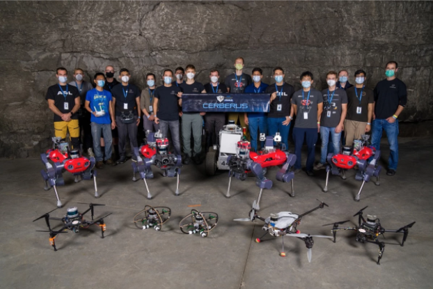
Team CERBERUS (CollaborativE walking and flying RoBots for autonomous ExploRation in Underground Settings) is a joint consortium between several universities and industrial organizations worldwide.
Figure 2. Team CERBERUS members with their multicopter drones, ANYmal C quadruped robots, and Super Mega Bot.
The team participated in the competition with four quadruped robots called ANYmal, five primarily in-house-built drones with variable size and payload capacity, and a rover robot in the form of Super Mega Bot. In the competition finals, the team ended up using four ANYmal robots and the Super Mega Bot for exploration and artifact detection.
Each ANYmal robot was equipped with two CPU-based computers and an NVIDIA Jetson AGX Xavier. The rover robot was equipped with an NVIDIA GTX 1070 GPU.
The CERBERUS team used a modified version of the You Only Look Once (YOLO) model for object detection. The model was trained on 40,000 labeled images using two NVIDIA RTX 3090 GPUs.
The trained model was further optimized using TensorRT before being deployed on Jetson for real-time inference. The Jetson AGX Xavier was able to perform inference at a collective rate of 20 Hz. In the competition finals, the CERBERUS team was the first to detect 23 of the 40 artifacts located in the environment, clinching the number one spot.
The CERBERUS team also used GPUs for the elevation mapping of the terrain and training the locomotion policy controller of the ANYmal quadruple robot. The elevation mapping was done in real-time using Jetson AGX Xavier. The ANYmal robot’s locomotion policy training for the rough terrain was done offline using desktop GPUs.
Team Co-STAR
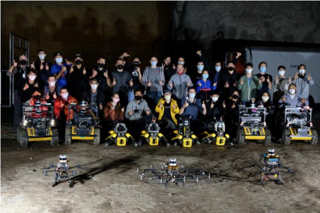
Led by researchers at NASA’s Jet Propulsion Laboratory (JPL) in Southern California along with other universities and industrial collaborators, team Collaborative SubTerranean Autonomous Robots (Co-STAR) was the winner of the 2020 competition focused on exploring complex underground urban environments.
Figure 3. Members of team Co-STAR with their robots (Spot, Husky, and drones).
They also successfully participated in the 2021 competition in mixed artificial and natural environments, placing fifth. The Co-STAR team entered the competition with four Spots, four Husky robots, and two drones.
Following an unexpected hardware issue in the final run, the team ended up using one Spot and three Husky robots. Each robot was equipped with a CPU-based computer along with one NVIDIA Jetson AGX Xavier.
For object detection, team Co-STAR used RGB and thermal images. They used the medium variant of the YOLO v5 model to process high-resolution images for real-time inference. The team trained two different models to perform inference on captured RGB and thermal images.
The image-based model was trained using approximately 54,000 labeled frames whereas the thermal image model was trained using about 2,400 labeled images. For training the model on their customized dataset, team Co-STAR used a pretrained YOLO v5 model on the COCO dataset and performed transfer learning using the NVIDIA Transfer Learning Toolkit (known as TAO Toolkit).
The models were trained using two on-premise NVIDIA A100 GPUs and an AWS instance that consisted of eight V100 GPUs. Before deploying the models on Jetson AGX Xavier, the team pruned the models using TensorRT.
Using this setup, team Co-STAR was able to perform inference at 28 Hz with RGB images received from five RealSense cameras and images received from one thermal camera. In the final run, the robots were able to detect all 13 artifacts present in the designated areas. The exploration time was limited due to the delayed deployment caused by unexpected hardware issues at the deployment site.
Equipped with the NVIDIA Jetson platform and NVIDIA GPU hardware, teams competing in the DARPA SubT event were able to effectively train models for real-time inference, addressing the challenge posed by underground environments with accurate object detection.
Posted by Abhijit Guha Roy, Research Software Engineer and Jie Ren, Research Scientist, Google Research
Deep machine learning (ML) systems have achieved considerable success in medical image analysis in recent years. One major contributing factor is access to abundant labeled datasets, which are used to train highly effective supervised deep learning models. However, in the real-world, these models may encounter samples exhibiting rare conditions that are individually too infrequent for per-condition classification. Nevertheless, such conditions can be collectively common because they follow a long-tail distribution and when taken together can represent a significant portion of cases — e.g., in a recent deep learning dermatological study, hundreds of rare conditions composed around 20% of cases encountered by the model at test time.
To prevent models from generating erroneous outputs on rare samples at test time, there remains a considerable need for deep learning systems with the ability to recognize when a sample is not a condition it can identify. Detecting previously unseen conditions can be thought of as an out-of-distribution (OOD) detection task. By successfully identifying OOD samples, preventive measures can be taken, like abstaining from prediction or deferring to a human expert.
Traditional computer vision OOD detection benchmarks work to detect dataset distribution shifts. For example, a model may be trained on CIFAR images but be presented with street view house numbers (SVHN) as OOD samples, two datasets with very different semantic meanings. Other benchmarks seek to detect slight differences in semantic information, e.g., between images of a truck and a pickup truck, or two different skin conditions. The semantic distribution shifts in such near-OOD detection problems are more subtle in comparison to dataset distribution shifts, and thus, are harder to detect.
The Near-OOD Dermatology Dataset We curated a near-OOD dermatology dataset that includes 26 inlier conditions, each of which are represented by at least 100 samples, and 199 rare conditions considered to be outliers. Outlier conditions can have as low as one sample per condition. The separation criteria between inlier and outlier conditions can be specified by the user. Here the cutoff sample size between inlier and outlier was 100, consistent with our previous study. The outliers are further split into training, validation, and test sets that are intentionally mutually exclusive to mimic real-world scenarios, where rare conditions shown during test time may have not been seen in training.
Long tail distribution of different dermatological conditions in our dataset. The 26 inlier conditions, with at least 100 samples, (blue) and the remaining 199 rare outlier conditions (orange). Outlier conditions can have as low as one sample per condition.
Train set
Validation set
Test set
Inlier
Outlier
Inlier
Outlier
Inlier
Outlier
Number of classes
26
68
26
66
26
65
Number of samples
8854
1111
1251
1082
1192
937
Inlier and outlier conditions in our benchmark dataset and detailed dataset split statistics. The outliers are further split into mutually exclusive train, validation, and test sets.
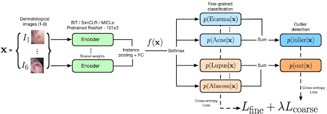
Hierarchical Outlier Detection Loss We propose to use “known outlier” samples during training that are leveraged to aid detection of “unknown outlier” samples during test time. Our novel hierarchical outlier detection (HOD) loss performs a fine-grained classification of individual classes for all inlier or outlier classes and, in parallel, a coarse-grained binary classification of inliers vs. outliers in a hierarchical setup (see the figure below). Our experiments confirmed that HOD is more effective than performing a coarse-grained classification followed by a fine-grained classification, as this could result in a bottleneck that impacted the performance of the fine-grained classifier.
We use the sum of the predictive probabilities of the outlier classes as the OOD score. As a primary OOD detection metric we use the area under receiver operating characteristics (AUROC) curve, which ranges between 0 and 1 and gives us a measure of separability between inliers and outliers. A perfect OOD detector, which separates all inliers from outliers, is assigned an AUROC score of 1. A popular baseline method, called reject bucket, separates each inlier individually from the outliers, which are grouped into a dedicated single abstention class. In addition to a fine-grained classification for each individual inlier and outlier classes, the HOD loss–based approach separates the inliers collectively from the outliers with a coarse-grained prediction loss, resulting in better generalization. While similar, we demonstrate that our HOD loss–based approach outperforms other baseline methods that leverage outlier data during training, achieving an AUROC score of 79.4% on the benchmark, a significant improvement over that of reject bucket, which achieves 75.6%.
Our model architecture and the HOD loss. The encoder (green) represents the wide ResNet 101×3 model pre-trained with different representation learning models (ImageNet, BiT, SimCLR, and MICLe; see below). The output of the encoder is sent to the HOD loss where fine-grained and coarse-grained predictions for inliers (blue) and outliers (orange) are obtained. The coarse predictions are obtained by summing over the fine-grained probabilities as indicated in the figure. The OOD score is defined as the sum of the probabilities of outlier classes.
Representation Learning and the Diverse Ensemble Strategy We also investigate how different types of representation learning help in OOD detection in conjunction with HOD by pretraining on ImageNet, BiT-L, SimCLR and MICLe models. We observe that including HOD loss improves OOD performance compared to the reject bucket baseline method for all four representation learning methods.
Representation Learning Methods
OOD detection metric (AUROC %)
With reject bucket
With HOD loss
ImageNet
74.7%
77%
BiT-L
75.6%
79.4%
SimCLR
75.2%
77.2%
MICLe
76.7%
78.8%
OOD detection performance for different representation learning models with reject bucket and with HOD loss.
Another orthogonal approach for improving OOD detection performance and accuracy is deep ensemble, which aggregates outputs from multiple independently trained models to provide a final prediction. We build upon deep ensemble, but instead of using a fixed architecture with a fixed pre-training, we combine different representation learning architectures (ImageNet, BiT-L, SimCLR and MICLe) and introduce objective loss functions (HOD and reject bucket). We call this a diverse ensemble strategy, which we demonstrate outperforms the deep ensemble for OOD performance and inlier accuracy.
Downstream Clinical Trust Analysis While we mainly focus on improving the performance for OOD detection, the ultimate goal for our dermatology model is to have high accuracy in predicting inlier and outlier conditions. We go beyond traditional performance metrics and introduce a “penalty” matrix that jointly evaluates inlier and outlier predictions for model trust analysis to approximate downstream impact. For a fixed confidence threshold, we count the following types of mistakes: (i) incorrect inlier predictions (i.e., mistaking inlier condition A as inlier condition B); (ii) incorrect abstention of inliers (i.e., abstaining from making a prediction for an inlier); and (iii) incorrect prediction for outliers as one of the inlier classes.
To account for the asymmetrical consequences of the different types of mistakes, penalties can be 0, 0.5, or 1. Both incorrect inlier and outlier-as-inlier predictions can potentially erode user trust in the model and were penalized with a score of 1. Incorrect abstention of an inlier as an outlier was penalized with a score of 0.5, indicating that potential model users should seek additional guidance given the model-expressed uncertainty or abstention. For correct decisions no cost is incurred, indicated by a score of 0.
Action of the Model
Prediction as Inlier
Abstain
Inlier
0 (Correct)
1 (Incorrect, mistakes that may erode trust)
0.5 (Incorrect, abstains inliers)
Outlier
1 (Incorrect, mistakes that may erode trust)
0 (Correct)
The penalty matrix is designed to capture the potential impact of different types of model errors.
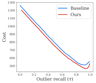
Because real-world scenarios are more complex and contain a variety of unknown variables, the numbers used here represent simplifications to enable qualitative approximations for the downstream impact on user trust of outlier detection models, which we refer to as “cost”. We use the penalty matrix to estimate a downstream cost on the test set and compare our method against the baseline, thereby making a stronger case for its effectiveness in real-world scenarios. As shown in the plot below, our proposed solution incurs a much lower estimated cost in comparison to baseline over all possible operating points.
Trust analysis comparing our proposed method to the baseline (reject bucket) for a range of outlier recall rates, indicated by 𝛕. We show that our method reduces downstream estimated cost, potentially reflecting improved downstream impact.
Conclusion In real-world deployment, medical ML models may encounter conditions that were not seen in training, and it’s important that they accurately identify when they do not know a specific condition. Detecting those OOD inputs is an important step to improving safety. We develop an HOD loss that leverages outlier data during training, and combine it with pre-trained representation learning models and a diverse ensemble to further boost performance, significantly outperforming the baseline approach on our new dermatology benchmark dataset. We believe that our approach, aligned with our AI Principles, can aid successful translation of ML algorithms into real-world scenarios. Although we have primarily focused on OOD detection for dermatology, most of our contributions are fairly generic and can be easily incorporated into OOD detection for other applications.
Acknowledgements We would like to thank Shekoofeh Azizi, Aaron Loh, Vivek Natarajan, Basil Mustafa, Nick Pawlowski, Jan Freyberg, Yuan Liu, Zach Beaver, Nam Vo, Peggy Bui, Samantha Winter, Patricia MacWilliams, Greg S. Corrado, Umesh Telang, Yun Liu, Taylan Cemgil, Alan Karthikesalingam, Balaji Lakshminarayanan, and Jim Winkens for their contributions. We would also like to thank Tom Small for creating the post animation.
Learn how edge computing is powering efficient energy operations, protecting worker health and safety, and improving power grid resiliency.
Each day, energy flows throughout our lives – from the fuel that powers cars and planes, to the gas used for stove top cooking, to the electricity that keeps the lights on in homes and businesses. Oil, gas, and electricity are mature commodity markets, but AI is transforming the processes used to produce, transport, and deliver these resources.
Enter AI deployed at the edge: on oil rigs, within power plants, riding along utility trucks, even embedded in smart buildings. Oil and gas enterprises and utilities are using AI and edge computing to improve operational efficiency, protect worker health and safety, integrate renewable energy, increase grid resiliency, and provide more reliable and affordable sources of energy to consumers.
Figure 1. Noteworthy AI, a member of NVIDIA Inception, put smart cameras on FirstEnergy’s trucks in a pilot that showed how edge computing can monitor millions of pole-mounted assets. Image courtesy of Noteworthy AI.
As companies and countries race to decarbonize and meet net-zero emissions goals, edge AI will play a key role managing distributed energy resources such as electric vehicles, home batteries, solar panels, and wind farms to enhance power grid resiliency and accelerate the energy transition. The following examples highlight the top AI use cases across the energy industry, including:
Software-defined smart grids: Future smart meters will use edge computing to optimize power flow, detect grid anomalies, deliver more reliable energy at a lower cost, and unlock opportunities for new energy applications. Utilidata, a leading grid-edge software company, is developing a software-defined smart grid chip with NVIDIA that will power next-generation smart meters to increase grid resiliency, decarbonization, and consumer value.
Autonomous operations: Industrial sites, such as oil rigs and power plants, require extensive monitoring for efficiency and safety because liquid, steam, or oil leakages can be catastrophic, costly, and wasteful. Global energy leaders, such as Siemens Energy, are using AI and machine learning to deliver a path to autonomous power plants. The company trains AI models using thousands of images and video streams from millions of onsite cameras and sensors to detect process anomalies. These models are deployed at the edge in power plants and use real-time inferencing to identify leaks. Rig operators are using computer vision, deep learning, and intelligent video analytics (IVA) to monitor heavy machinery, detect potential hazards, and alert workers in real-time to protect their health and safety, prevent accidents, and assign repair technicians for maintenance.
Pipeline optimization: Oil and gas enterprises rely on finding the best-fit routes to transfer oil to refineries and eventually fuel stations. Edge AI can calculate the optimal flow of oil to ensure reliability of production and protect long-term pipeline health. Using IVA, these companies can inspect pipelines for defects that could lead to dangerous failures and automatically alert pipeline operators. Further downstream, NVIDIA ReOpt uses GPU-accelerated solvers for logistics and route optimization, which can efficiently route fuel to fueling stations.
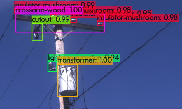
Power grid maintenance: With proactive maintenance, utilities can accurately detect defects and reduce unplanned outages to better serve customers. FirstEnergy worked with Noteworthy AI, a NVIDIA Inception member, on a pilot project to automate utility pole inspections. Fixed camera systems powered by NVIDIA Jetson were secured to the roof of service trucks and collected standardized, high-resolution images of their utility poles, power lines, and pole-mounted assets. The images were analyzed at the edge to determine if repairs or vegetation management was needed. Edge computing can help monitor the estimated 185 million utility poles in the United States, and reduce the tens of millions of dollars spent each year by utilities to manually track and maintain poles.
Power grid simulation: Intelligent forecasting using GPU-accelerated grid simulations combined with historical data on energy usage and weather can inform more efficient generation, distribution, and management of energy resources to consumers. AI helps manage the bidirectional flow of power in a grid, delivering reliable energy to residents and enterprises while automating the process for consumers to sell their additional energy back to the grid.
Thanks to edge AI, the future of energy is more sustainable than ever. Explore how NVIDIA is building an ecosystem to accelerate the energy transition.
GeForce NOW is taking cloud gaming to new heights. This GFN Thursday delivers an upgraded streaming experience as part of an update that is now available to all members. It includes new resolution upscaling options to make members’ gaming experiences sharper, plus the ability to customize streaming settings in session. The GeForce NOW app is Read article >

 cuFFTMp is a multi-node, multi-process extension to cuFFT that enables scientists and engineers to solve challenging problems on exascale platforms.
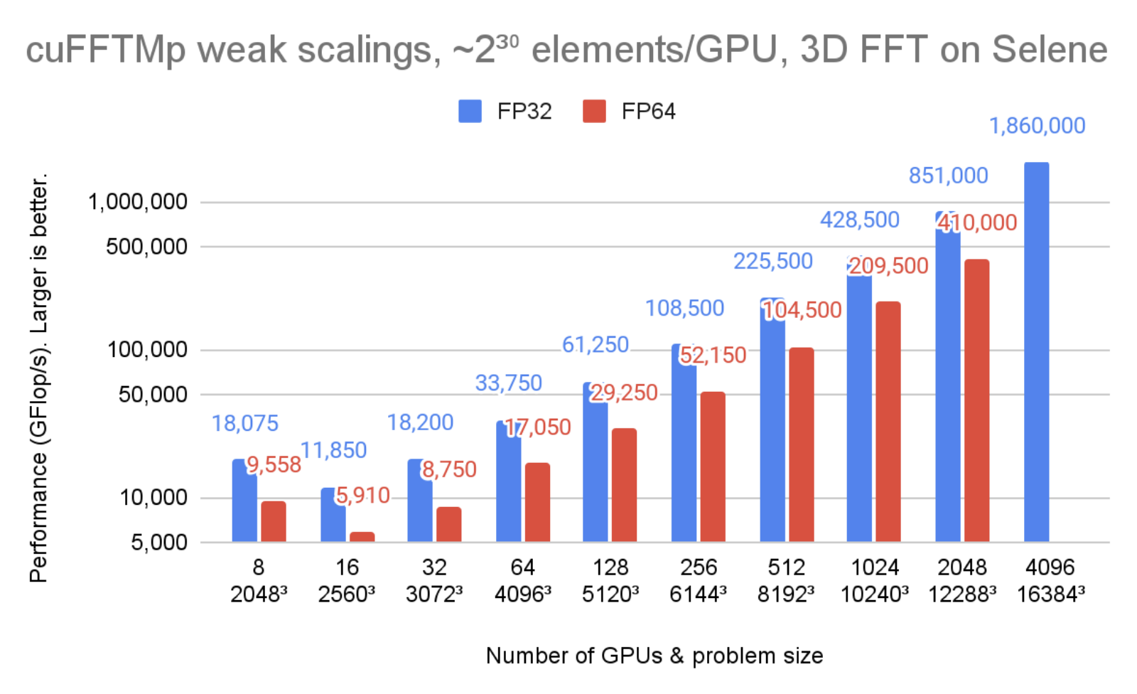
 Meta’s AI supercomputer — the largest NVIDIA DGX A100 customer system to date — will deliver 5 exaflops of AI performance.
 Nsight Compute kernel profiler now includes Range Replay, Memory Analysis, and Guided Analysis enhancements.
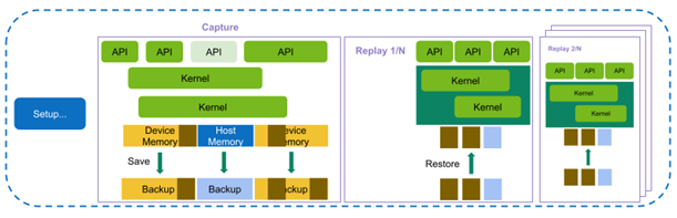
 With NVIDIA Jetson embedded platforms, teams at the DARPA SubT Challenge detected objects with both high accuracy and high throughput.
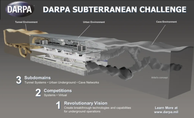


 Learn how edge computing is powering efficient energy operations, protecting worker health and safety, and improving power grid resiliency.