Posted by Sergio Orts Escolano and Jana Ehman, Software Engineers, Google Research
Image matting is the process of extracting a precise alpha matte that separates foreground and background objects in an image. This technique has been traditionally used in the filmmaking and photography industry for image and video editing purposes, e.g., background replacement, synthetic bokeh and other visual effects. Image matting assumes that an image is a composite of foreground and background images, and hence, the intensity of each pixel is a linear combination of the foreground and the background.
In the case of traditional image segmentation, the image is segmented in a binary manner, in which a pixel either belongs to the foreground or background. This type of segmentation, however, is unable to deal with natural scenes that contain fine details, e.g., hair and fur, which require estimating a transparency value for each pixel of the foreground object.
Alpha mattes, unlike segmentation masks, are usually extremely precise, preserving strand-level hair details and accurate foreground boundaries. While recent deep learning techniques have shown their potential in image matting, many challenges remain, such as generation of accurate ground truth alpha mattes, improving generalization on in-the-wild images and performing inference on mobile devices treating high-resolution images.
With the Pixel 6, we have significantly improved the appearance of selfies taken in Portrait Mode by introducing a new approach to estimate a high-resolution and accurate alpha matte from a selfie image. When synthesizing the depth-of-field effect, the usage of the alpha matte allows us to extract a more accurate silhouette of the photographed subject and have a better foreground-background separation. This allows users with a wide variety of hairstyles to take great-looking Portrait Mode shots using the selfie camera. In this post, we describe the technology we used to achieve this improvement and discuss how we tackled the challenges mentioned above.
 |
| Portrait Mode effect on a selfie shot using a low-resolution and coarse alpha matte compared to using the new high-quality alpha matte. |
Portrait Matting
In designing Portrait Matting, we trained a fully convolutional neural network consisting of a sequence of encoder-decoder blocks to progressively estimate a high-quality alpha matte. We concatenate the input RGB image together with a coarse alpha matte (generated using a low-resolution person segmenter) that is passed as an input to the network. The new Portrait Matting model uses a MobileNetV3 backbone and a shallow (i.e., having a low number of layers) decoder to first predict a refined low-resolution alpha matte that operates on a low-resolution image. Then we use a shallow encoder-decoder and a series of residual blocks to process a high-resolution image and the refined alpha matte from the previous step. The shallow encoder-decoder relies more on lower-level features than the previous MobileNetV3 backbone, focusing on high-resolution structural features to predict final transparency values for each pixel. In this way, the model is able to refine an initial foreground alpha matte and accurately extract very fine details like hair strands. The proposed neural network architecture efficiently runs on Pixel 6 using Tensorflow Lite.
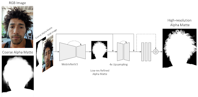 |
| The network predicts a high-quality alpha matte from a color image and an initial coarse alpha matte. We use a MobileNetV3 backbone and a shallow decoder to first predict a refined low-resolution alpha matte. Then we use a shallow encoder-decoder and a series of residual blocks to further refine the initially estimated alpha matte. |
Most recent deep learning work for image matting relies on manually annotated per-pixel alpha mattes used to separate the foreground from the background that are generated with image editing tools or green screens. This process is tedious and does not scale for the generation of large datasets. Also, it often produces inaccurate alpha mattes and foreground images that are contaminated (e.g., by reflected light from the background, or “green spill”). Moreover, this does nothing to ensure that the lighting on the subject appears consistent with the lighting in the new background environment.
To address these challenges, Portrait Matting is trained using a high-quality dataset generated using a custom volumetric capture system, Light Stage. Compared with previous datasets, this is more realistic, as relighting allows the illumination of the foreground subject to match the background. Additionally, we supervise the training of the model using pseudo–ground truth alpha mattes from in-the-wild images to improve model generalization, explained below. This ground truth data generation process is one of the key components of this work.
Ground Truth Data Generation
To generate accurate ground truth data, Light Stage produces near-photorealistic models of people using a geodesic sphere outfitted with 331 custom color LED lights, an array of high-resolution cameras, and a set of custom high-resolution depth sensors. Together with Light Stage data, we compute accurate alpha mattes using time-multiplexed lights and a previously recorded “clean plate”. This technique is also known as ratio matting.
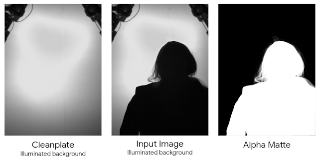 |
| This method works by recording an image of the subject silhouetted against an illuminated background as one of the lighting conditions. In addition, we capture a clean plate of the illuminated background. The silhouetted image, divided by the clean plate image, provides a ground truth alpha matte. |
Then, we extrapolate the recorded alpha mattes to all the camera viewpoints in Light Stage using a deep learning–based matting network that leverages captured clean plates as an input. This approach allows us to extend the alpha mattes computation to unconstrained backgrounds without the need for specialized time-multiplexed lighting or a clean background. This deep learning architecture was solely trained using ground truth mattes generated using the ratio matting approach.
 |
| Computed alpha mattes from all camera viewpoints at the Light Stage. |
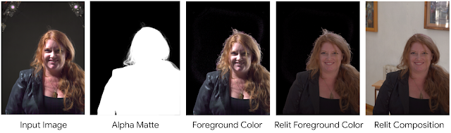
Leveraging the reflectance field for each subject and the alpha matte generated with our ground truth matte generation system, we can relight each portrait using a given HDR lighting environment. We composite these relit subjects into backgrounds corresponding to the target illumination following the alpha blending equation. The background images are then generated from the HDR panoramas by positioning a virtual camera at the center and ray-tracing into the panorama from the camera’s center of projection. We ensure that the projected view into the panorama matches its orientation as used for relighting. We use virtual cameras with different focal lengths to simulate the different fields-of-view of consumer cameras. This pipeline produces realistic composites by handling matting, relighting, and compositing in one system, which we then use to train the Portrait Matting model.
 |
| Composited images on different backgrounds (high-resolution HDR maps) using ground truth generated alpha mattes. |
Training Supervision Using In-the-Wild Portraits
To bridge the gap between portraits generated using Light Stage and in-the-wild portraits, we created a pipeline to automatically annotate in-the-wild photos generating pseudo–ground truth alpha mattes. For this purpose, we leveraged the Deep Matting model proposed in Total Relighting to create an ensemble of models that computes multiple high-resolution alpha mattes from in-the-wild images. We ran this pipeline on an extensive dataset of portrait photos captured in-house using Pixel phones. Additionally, during this process we performed test-time augmentation by doing inference on input images at different scales and rotations, and finally aggregating per-pixel alpha values across all estimated alpha mattes.
Generated alpha mattes are visually evaluated with respect to the input RGB image. The alpha mattes that are perceptually correct, i.e., following the subject’s silhouette and fine details (e.g., hair), are added to the training set. During training, both datasets are sampled using different weights. Using the proposed supervision strategy exposes the model to a larger variety of scenes and human poses, improving its predictions on photos in the wild (model generalization).
 |
| Estimated pseudo–ground truth alpha mattes using an ensemble of Deep Matting models and test-time augmentation. |
Portrait Mode Selfies
The Portrait Mode effect is particularly sensitive to errors around the subject boundary (see image below). For example, errors caused by the usage of a coarse alpha matte keep sharp focus on background regions near the subject boundaries or hair area. The usage of a high-quality alpha matte allows us to extract a more accurate silhouette of the photographed subject and improve foreground-background separation.
Try It Out Yourself
We have made front-facing camera Portrait Mode on the Pixel 6 better by improving alpha matte quality, resulting in fewer errors in the final rendered image and by improving the look of the blurred background around the hair region and subject boundary. Additionally, our ML model uses diverse training datasets that cover a wide variety of skin tones and hair styles. You can try this improved version of Portrait Mode by taking a selfie shot with the new Pixel 6 phones.
 |
| Portrait Mode effect on a selfie shot using a coarse alpha matte compared to using the new high quality alpha matte. |
Acknowledgments
This work wouldn’t have been possible without Sergio Orts Escolano, Jana Ehmann, Sean Fanello, Christoph Rhemann, Junlan Yang, Andy Hsu, Hossam Isack, Rohit Pandey, David Aguilar, Yi Jinn, Christian Hane, Jay Busch, Cynthia Herrera, Matt Whalen, Philip Davidson, Jonathan Taylor, Peter Lincoln, Geoff Harvey, Nisha Masharani, Alexander Schiffhauer, Chloe LeGendre, Paul Debevec, Sofien Bouaziz, Adarsh Kowdle, Thabo Beeler, Chia-Kai Liang and Shahram Izadi. Special thanks to our photographers James Adamson, Christopher Farro and Cort Muller who took numerous test photographs for us.

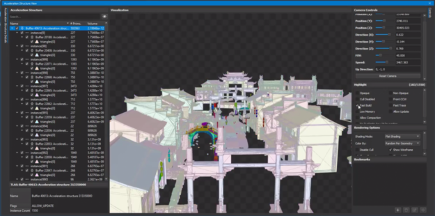
 The latest Nsight Graphics 2022.1 release supports Direct3D (11, 12, DXR), Vulkan 1.3, ray tracing extension, OpenGL, OpenVR, and the Oculus SDK.
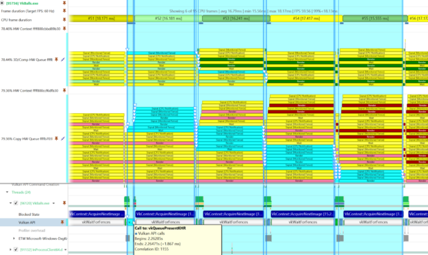
 The latest release of Vulkan 1.3 simplifies render passes and makes synchronization easier.